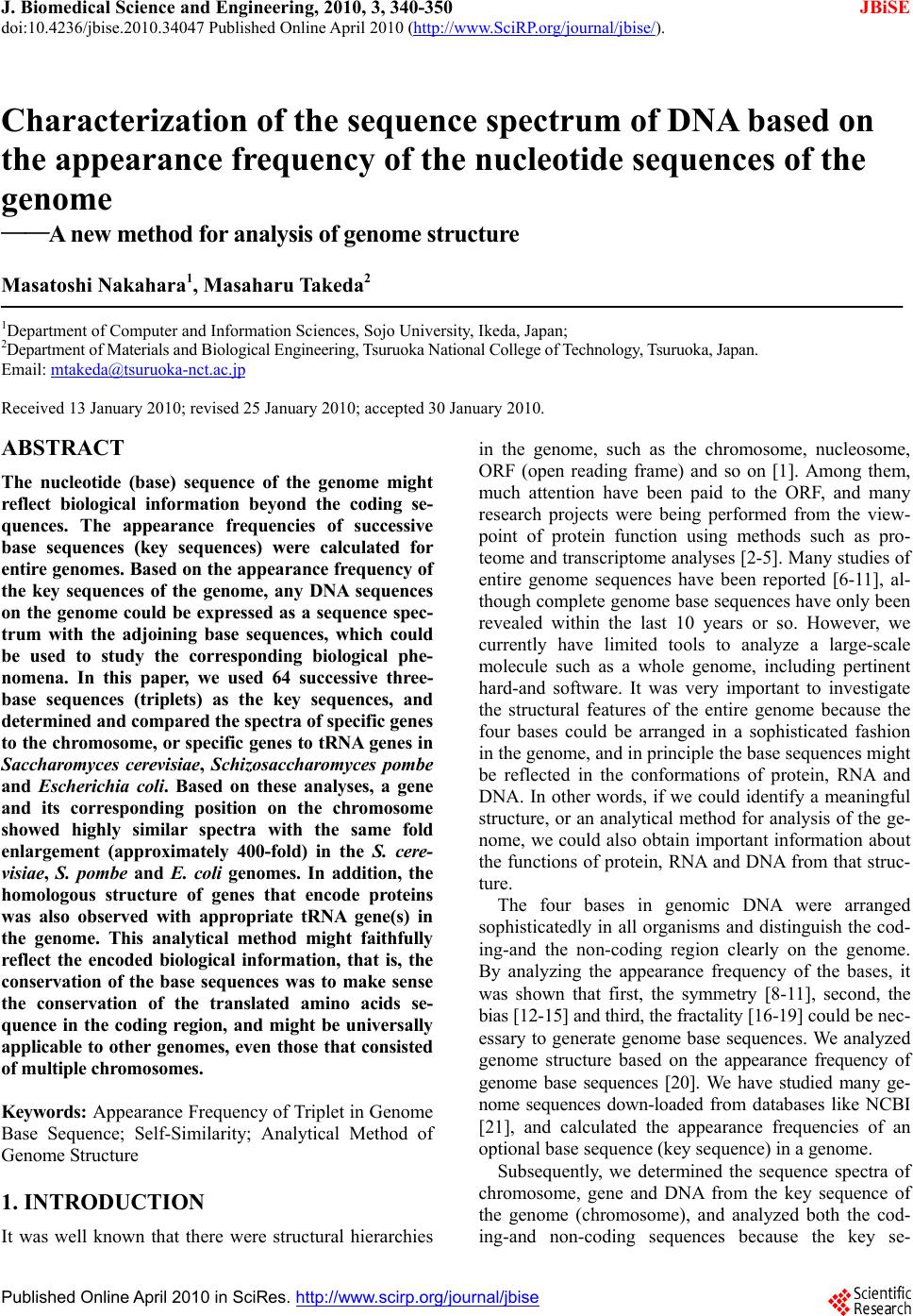J. Biomedical Science and Engineering, 2010, 3, 340-350 JBiSE
doi:10.4236/jbise.2010.34047 Published Online April 2010 (http://www.SciRP.org/journal/jbise/).
Published Online April 2010 in SciRes. http://www.scirp.org/journal/jbise
Characterization of the sequence spectrum of DNA based on
the appearance frequency of the nucleotide sequences of the
genome
——A new method for analysis of genome structur e
Masatoshi Nakahara1, Masaharu Takeda2
1Department of Computer and Information Sciences, Sojo University, Ikeda, Japan;
2Department of Materials and Biological Engineering, Tsuruoka National College of Technology , Tsuruoka, Japan.
Received 13 January 2010; revised 25 January 2010; accepted 30 January 2010.
ABSTRACT
The nucleotide (base) sequence of the genome might
reflect biological information beyond the coding se-
quences. The appearance frequencies of successive
base sequences (key sequences) were calculated for
entire genomes. Based on the appearance frequency of
the key sequences of the genome, any DNA sequences
on the genome could be expressed as a sequence spec-
trum with the adjoining base sequences, which could
be used to study the corresponding biological phe-
nomena. In this paper, we used 64 successive three-
base sequences (triplets) as the key sequences, and
determined and compared the spectra of specific genes
to the chromosome, or specific genes to tRNA genes in
Saccharomyces cerevisiae, Schizosaccharomyces pombe
and Escherichia coli. Based on these analyses, a gene
and its corresponding position on the chromosome
showed highly similar spectra with the same fold
enlargement (approximately 400-fold) in the S. cere-
visiae, S. pombe and E. coli genomes. In addition, the
homologous structure of genes that encode proteins
was also observed with appropriate tRNA gene(s) in
the genome. This analytical method might faithfully
reflect the encoded biological information, that is, the
conservation of the base sequences was to make sense
the conservation of the translated amino acids se-
quence in the coding region, and might be universally
applicable to other genomes, even those that consisted
of multiple chromosomes.
Keywords: Appearance Frequency of Triplet in Genome
Base Sequence; Self-Similarity; Analytical Method of
Genome Structure
1. INTRODUCTION
It was well known that there were structural hierarchies
in the genome, such as the chromosome, nucleosome,
ORF (open reading frame) and so on [1]. Among them,
much attention have been paid to the ORF, and many
research projects were being performed from the view-
point of protein function using methods such as pro-
teome and transcriptome analyses [2-5]. Many studies of
entire genome sequences have been reported [6-11], al-
though complete genome base sequences have only been
revealed within the last 10 years or so. However, we
currently have limited tools to analyze a large-scale
molecule such as a whole genome, including pertinent
hard-and software. It was very important to investigate
the structural features of the entire genome because the
four bases could be arranged in a sophisticated fashion
in the genome, and in principle the base sequences might
be reflected in the conformations of protein, RNA and
DNA. In other words, if we could identify a meaningful
structure, or an analytical method for analysis of the ge-
nome, we could also obtain important information about
the functions of protein, RNA and DNA from that struc-
ture.
The four bases in genomic DNA were arranged
sophisticatedly in all organisms and distinguish the cod-
ing-and the non-coding region clearly on the genome.
By analyzing the appearance frequency of the bases, it
was shown that first, the symmetry [8-11], second, the
bias [12-15] and third, the fractality [16-19] could b e n e c-
essary to generate genome base sequences. We analyzed
genome structure based on the appearance frequency of
genome base sequences [20]. We have studied many ge-
nome sequences down-loaded from databases like NCBI
[21], and calculated the appearance frequencies of an
optional base sequence (key sequence) in a genome.
Subsequently, we determined the sequence spectra of
chromosome, gene and DNA from the key sequence of
the genome (chromosome), and analyzed both the cod-
ing-and non-coding sequences because the key se-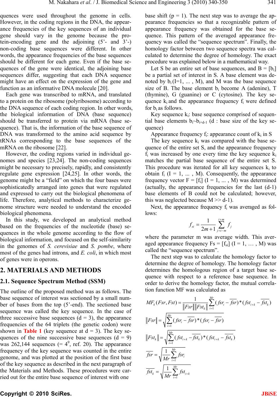

M. Nakahara et al. / J. Biomedical Science and Engineering 3 (2010) 340-350 341
quences were used throughout the genome in cells.
However, in the coding regions in the DNA, the appear-
ance frequencies of the key sequences of an individual
gene should vary in the genome because the pro-
tein-encoding gene and the adjoining (5’- and 3’-)
non-coding base sequences were different. In other
words, the appearance frequencies of the base sequences
should be different for each gene. Even if the base se-
quences of the gene were identical, the adjoining base
sequences differ, suggesting that each DNA sequence
might have an effect on the expression of the gene and
function as an informative DNA molecule [20].
Each gene was transcribed to mRNA, and translated
to a protein on the ribosome (polyribosome) according to
the DNA sequence of each coding region. In other words,
the biological information of DNA (base sequence)
should be transferred to protein via mRNA (base se-
quence). That is, the information of the base sequence of
DNA was transformed to the amino acid sequence by
tRNAs corresponding to the base sequences of the
mRNA on the ribosome [22].
However, the coding regions varied in individual ge-
nomes and species [23,24]. The non-coding sequences
might be necessary to precisely, rapidly, and consistently
regulate gene expression [24,25]. In other words, the
genome might be a “field” on which the four bases were
sophisticatedly arranged into genes that were regulated
and expressed to carry out the biological phenomena of
life. Therefore, analytical methods to characterize ge-
nome structure were needed to understand the encoded
biologic al phenom e na .
In this study, we developed an analytical method
based on the frequencies of the nucleotide (base) se-
quences in the whole genome according to the flow of
biological information, and focused on the self-similarity
in the genomes of S. cerevisiae and S. pombe, where
most of the genes had introns, and E. coli, in which most
of genes were in operons.
2. MATERIALS AND METHODS
2.1. Sequence Spectrum Method (SSM)
The outline of the proposed method was as follows. The
base sequence of interest was sectioned by a small num-
ber of bases from the top (5’-end). The sectioned base
sequence was called the key sequence. In the case of
three successive base sequences (d = 3), the appearance
frequencies of the 64 triplets (the genetic codon) were
shown in Ta b l e 1 (key sequence at d = 3). The key se-
quences of the nine successive base sequences (d = 9)
was 262,144 sequences (= 49, ref. 20). The appearance
frequency of the key sequence was counted in the entire
genome, and was plotted at the position of the first base
of the key sequence as described in the next pa ragraph of
the Materials and Methods. These procedures were car-
ried out for the entire base sequence of interest with one
base shift (p = 1). The next step was to average the ap-
pearance frequencies so that a recognizable pattern of
appearance frequency was obtained for the base se-
quence. This pattern of the averaged appearance fre-
quency was called the “sequence spectrum”. Finally, the
homology factor between two sequence spectra was cal-
culated to determine the degree of homology. The exact
procedure was explained below in a mathematic al way.
Let S be an entire set of base sequences, and B = [bi]
be a partial set of interest in S. A base element was de-
noted by bi (I=1, ... , M), and M was the base sequence
size of B. The base element bi become A (adenine), T
(thymine), G (guanine) or C (cytosine). The key se-
quence ki and the appearance frequency fi were defined
for bi as follows.
Key sequence ki: base sequence comprised of sequen-
tial base elements bi~bi+d-1 (d : base size of the key se-
quence)
Appearance frequency fi: appearance count of ki in S
The key sequence ki was compared with the base se-
quence of the entire set S, and the appearance frequency
fi was increased by one every time the key sequence ki
matches the partial base sequence of the entire set S.
This procedure was iterated for all key sequences ki to
obtain fi (I = 1, ... , M). Consequently, the appearance
frequency vector F = [fi] (I = 1, ... , M) was determined
(actually, the appearance frequencies for the last (d-1)
base elements of B could not be calculated; however,
this was neglected because M >> d-1).
Next, the appearance frequency fi was averaged as fol-
lows: 1
21
im
s
ij
jim
f
f
m



where the parameter m was average width. This aver-
aged appearance frequency Fs = [fsi] (I = 1, … , M) was
called the “sequence spectrum”.
The next step was to calculate the homology factor to
determine the degree of homology. The homology factor
determines the homologous region of a target base se-
quence with respect to a reference base sequence. In
order to derive the homology factor, the mutual correla-
tion function MF was calculated as
1
1
1
1
1
1
(,)( )*()
()*()
()*()
1
1
Mr
kiikk
i
k
Mr
ii
i
Mr
kikkikk
i
Mr
i
i
Mr
kik
i
M
FFsr Fstfsrfsrfstfst
Fsr Fst
Fsrfsr fsrfsr fsr
Fstfst fstfstfst
fsr fsr
Mr
fst fst
Mr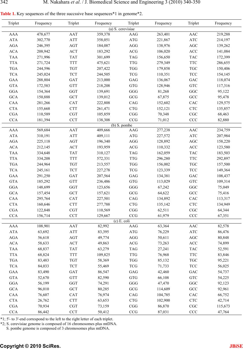









 
 








M. Nakahara et al. / J. Biomedical Science and Engineering 3 (2010) 340-350 342
Table 1. Key sequences of the three succssive base sequences*1 in genome*2.
Triplet Frequency Triplet Frequency Triplet Frequency Triplet Frequency
(a) S. cerevisiae
AAA 478,677 AAT 359,378 AAG 263,401 AAC 219,288
ATA 302,770 ATT 358,051 ATG 221,867 ATC 214,197
AGA 246,395 AGT 184,087 AGG 138,976 AGC 139,262
ACA 208,942 ACT 183,292 ACG 106,020 ACC 141,084
TAA 271,996 TAT 301,699 TAG 156,650 TAC 172,399
TTA 271,724 TTT 475,621 TTG 279,349 TTC 286,655
TGA 244,596 TGT 207,422 TGG 179,858 TGC 150,406
TCA 245,024 TCT 244,505 TCG 110,351 TCC 154,145
GAA 288,804 GAT 213,000 GAG 136,067 GAC 118,074
GTA 172,583 GTT 218,208 GTG 128,946 GTC 117,316
GGA 154,364 GGT 139,691 GGG 81,268 GGC 95,122
GCA 150,888 GCT 139,012 GCG 67,875 GCC 95,478
CAA 281,266 CAT 222,808 CAG 152,602 CAC 129,575
CTA 155,668 CTT 261,471 CTG 152,121 CTC 135,857
CGA 110,589 CGT 105,859 CGG 70,348 CGC 68,463
CCA 181,394 CCT 138,308 CCG 71,012 CCC 82,880
(
b
)
S.
p
ombe
AAA 569,684 AAT 409,666 AAG 277,238 AAC 234,759
ATA 310,191 ATT 409,111 ATG 227,572 ATC 207,984
AGA 225,118 AGT 196,340 AGG 128,892 AGC 158,220
ACA 212,145 ACT 193,959 ACG 110,332 ACC 123,580
TAA 334,648 TAT 310,127 TAG 162,059 TAC 183,503
TTA 334,208 TTT 572,331 TTG 296,280 TTC 292,897
TGA 244,964 TGT 213,557 TGG 156,002 TGC 157,500
TCA 245,161 TCT 227,278 TCG 123,339 TCC 149,364
GAA 291,250 GAT 207,564 GAG 134,381 GAC 108,437
GTA 185,292 GTT 236,486 GTG 113,029 GTC 109,314
GGA 148,699 GGT 123,656 GGG 67,242 GGC 75,049
GCA 157,454 GCT 157,621 GCG 64,622 GCC 75,416
CAA 295,764 CAT 227,501 CAG 134,892 CAC 113,317
CTA 160,646 CTT 277,788 CTG 135,142 CTC 134,949
CGA 122,848 CGT 110,569 CGG 62,511 CGC 64,344
CCA 156,714 CCT 129,667 CCG 61,979 CCC 67,351
(
c
)
E. coli
AAA 108,901 AAT 82,992 AAG 63,364 AAC 82,578
ATA 63,692 ATT 83,395 ATG 76,229 ATC 86,476
AGA 56,618 AGT 49,774 AGG 50,611 AGC 80,848
ACA 58,633 ACT 49,863 ACG 73,263 ACC 74,899
TAA 68,837 TAT 63,279 TAG 27,241 TAC 52,591
TTA 68,824 TTT 109,825 TTG 76,968 TTC 83,846
TGA 83,483 TGT 58,369 TGG 85,132 TGC 95,221
TCA 84,033 TCT 55,469 TCG 71,733 TCC 56,025
GAA 83,490 GAT 86,547 GAG 42,460 GAC 54,737
GTA 52,670 GTT 82,590 GTG 66,108 GTC 54,225
GGA 56,199 GGT 74,291 GGG 47,470 GGC 92,123
GCA 96,010 GCT 80,285 GCG 114,609 GCC 92,961
CAA 76,607 CAT 76,974 CAG 104,785 CAC 66,752
CTA 26,762 CTT 63,653 CTG 102,900 CTC 42,714
CGA 70,934 CGT 73,159 CGG 86,870 CGC 115,673
CCA 86,442 CCT 50,412 CCG 87,031 CCC 47,764
*1; 5'- to 3'-end correspond to the left to the right letter of each triplet.
*2; S. cerevisiae g e nome is composed of 16 c hromosomes pl us mtDNA.
S. pombe genome is composed of 3 chromosomes plus mtDNA.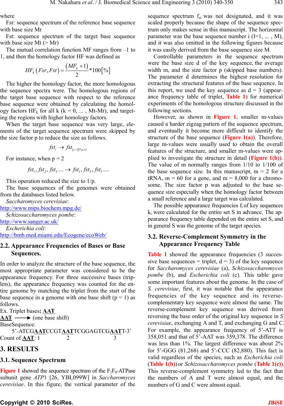

M. Nakahara et al. / J. Biomedical Science and Engineering 3 (2010) 340-350 343
where
Fsr: sequence spectrum of the reference base sequence
with base size Mr
Fst: sequence spectrum of the target base sequence
with base size Mt (> Mr)
The mutual correlation function MF ranges from –1 to
1, and then the homology factor HF was defined as



1
,*100 %
2
k
k
MF
HFFsr Fst 
The higher the homology factor, the more homologous
the sequence spectra were. The homologous regions of
the target base sequence with respect to the reference
base sequence were obtained by calculating the homol-
ogy factors HFk for all k (k = 0, ... , Mt-Mr), and target-
ing the regions with hi g he r ho mology factors .
When the target base sequence was very large, ele-
ments of the target sequence spectrum were skipped by
the size factor p to reduce the size as follows.

1* 1
iip
fst fst



For instance, when p = 2
123 135
,, ,,
f
st fstfstfst fstfst
This operation reduced the size to 1/p.
The base sequences of the genomes were obtained
from the databases listed below.
Saccharomyces cerevisiae:
http://www.mips.biochem.mpg.de/
Schizosaccharomyces pombe:
http://www.sanger.ac.uk /
Escherichia coli:
http://bmb.med.miami.ed u/Eco gene/ecoWeb /
2.2. Appearance Frequencies of Bases or Base
Sequences.
In order to analyze the structure of the base sequence, the
most appropriate parameter was considered to be the
appearance frequency. For three successive bases (trip-
lets), the appearance frequency was counted for the en-
tire genome by matching the triplet from the start of the
base sequence in a genome with one base shift (p = 1) as
follows.
Ex. T riplet bases: AAT
AAT (one base shift)
BaseSequence:
5’-ATCGAATCCGTAATTCGGAGTCGAATT-3’
Count of AAT: 1 2 3
3. RESULTS
3.1. Sequence Spectrum
Figure 1 showed the sequen ce spectrum of the F1F0-ATPase
subunit gene ATP1 [26, YBL099W] in Saccharomyces
cerevisiae. In this figure, the vertical parameter of the
sequence spectrum fsi was not designated, and it was
scaled properly because the shape of the sequence spec-
trum only makes sense in this manuscript. The horizontal
parameter was the base sequence number i (I=1, ... , M),
and it was also omitted in the following figures because
it was easily derived from the base sequence size M.
Controllable parameters in the sequence spectrum
were the base size d of the key sequence, the average
width m, and the size factor p (skipped base numbers).
The parameter d determines the highest resolution for
extracting the structural features of the base sequence. In
this report, we used the key sequence as d = 3 (appear-
ance frequency table of triplet, Table 1) for numerical
experiments of the homologous structure discussed in the
following sections.
However, as shown in Figure 1, smaller m-values
caused a harder zigzag pattern of the sequence spectrum,
and eventually it become more difficult to identify the
structure of the base sequence (Figure 1(a)). Therefore,
large m-values were usually used to obtain the overall
features of the structure, and smaller m-values were ap-
plied to investigate the structure in detail (Figure 1(b)).
The value of m normally ranges from 1/10 to 1/100 of
the base sequence size. In this manuscript, m = 2 for a
tRNA, m = 60 for a gene, and m = 8,000 for a chromo-
some. The size factor p was adjusted to the base se-
quence size especially when the homology factor between
a small reference and a large target was calculated.
The possible appearance frequencies fi of ke y sequences
ki were calculated for the entire set S in advance. The ap-
pearance frequency table depended on the entire set S, and
in general S was the genome of the t arget spec i es .
3.2. Reverse-Complement Symmetry in the
Appearance Frequency Table
Table 1 showed the appearance frequencies (3 succes-
sive base sequences = triplet, d = 3) of the key sequence
for Saccharomyces cerevisiae (a), Schizosaccharomyces
pombe (b), and Escherichia coli (c). This table gave
some important features about the genome. In the case of
S. cerevisiae, first, it was notable that the appearance
frequencies of the key sequence and its reverse-
complementary key sequence were almost the same. The
reverse-complement key sequence was derived from
reversing the base order of the original key sequence in S.
cerevisiae, exchanging A and T, and exchanging G and C.
For example, the appearance frequency of 5’-ATT is
358,051 an d that of 5’-A AT was 359,378. The difference
was less than 1%. The largest difference was about 2%
for 5’-GGG (81,268) and 5’-CCC (82,880). This fact is
valid regardless of the species, such as Escherichia coli
(Table 1(b)) or Schizosaccharomyces pombe (Table 1(c)).
This reverse-complement symmetry led to the fact that
the numbers of A and T were almost equal, and the
number s of G and C we r e almost equ a l.

M. Nakahara et al. / J. Biomedical Science and Engineering 3 (2010) 340-350 344
(a) ATP1, m = 0
(b) ATP1, m = 60
Figure 1. Sequence spectrum of ATP1. Sequence spectra of
AT P1 [26-28] from Saccharomyces cerevisiae with different
average widths (a) m = 0, and (b) m = 60. The vertical parame-
ter (appearance frequency of the triplet, d = 3) of the sequence
spectrum is not designated, and it is scaled properly. The hori-
zontal axis is the base sequence of AT P1 (1,638 nt designated
as M, ATG = start codon – TAA = stop codon). The skipped
base numbers (p) are shown in the figures. The zigzag motif
becomes more moderate and the resolution becomes lower as
the average width of m becomes larger.
Generally it was well known that the numbers of A
and T and the numbers of G and C were the same due to
the double helix structure of DNA. However, in this case,
this coincidence of base numbers occurred in the genome,
so it had nothing to do with the double helix structure.
Therefore, the coincidence of base numbers occurred
when the base sequence size was very large even in a sin-
gle strand. Actually this reverse-complement symmetry
occurred in each chromosome as well.
On the other hand, it did not occur when the base se-
quence size was not large enough. For instance, the base
sequence size of a single gene was not adequate. The fact
that the appearance frequencies of the key sequence and
its reverse-complementary key sequence were almost
equal implies that there must be a certain amount of
symmetry in the genome.
Second, the appearance frequency (in parentheses) for
each key sequence was not random, but some of the key
sequences had very close appearance frequencies even
when they did not have a complementary relationship.
For example, in the case of S. cerevisiae, the key se-
quences 5’-AAC (219,288), 5’-ATC (214,197) and
5’-ACA (208,942) had close appearance frequencies of
about 210,000, and those of the key sequences 5’-ACG
(106,020), 5’-CGA (110,589) and 5’-GAC (110,874)
were about 110,000. These different key sequences with
close appearance frequencies might have a similar effect
on the sequence spectrum. In other words, sin-
gle-stranded DNA with base-symmetry might be able to
make many double-helical stems in a molecule, and the
peaks of the sequence spectrum, the “up” of the dou-
ble-helical stem might have the same effect on the
“down” of it. Needless to say, these facts were valid re-
gardless of the species.
3.3. Homologous Structure in Genomes
(Enlargement-Reduction of the base Sequence)
ATP1 (YBL099W) of S. cerevisiae was present on the
left arm of chromosome II (37,045-38,679 from the left
telomere). Figure 2 showed the spectra of ATP1 (1,638
nt, Figure 1(b)), and (a) chromosome II (813,139 nt),
respectively. The red arrowhead indicated the position of
ATP1 on chromoso me II [27, 28]. When the spectrum of
ATP1 (1,638 nt) was skipped 3 bases and the homology
analyzed between chromosome II and the skipped-ATP1,
the red-region (20,401 ~ 60,401 = 40,000 nt) of chromo-
some II was homologous to the 3 bases-skipped-ATP1
(1,341 ~ 1,638 = 297 nt) (Figure 2(b), HF of the
red-region of chromosome II to the purple-region of
ATP1 = 95%).
When ATP1 was skipped 10, or 16 bases, the ho-
mologous area of ATP1 to the red-region of chromosome
II was enlarged to 990 nt (Figure 2(c), 648 ~ 1,638), or
1,584 nt (Figure 2(d), 54 ~ 1,638), r espectively. That is,
the base sequence of the complete ATP1 gene had
self-similarity to the gene-position on chromosome II.
Other genes of S. cerevisiae were highly homologous
with the gene-position of each chromosome irrespective
to the sizes, the order, the direction of transcription and
the chromosomes. The fold-enlargement of the gene to
each chromosome was calculated as approximately
400-fold (Table 2(a)).
The same relationship of the enlargement-reduction of
the chromosome-gene was observed in S. pombe (eu-
karyotic cells, Tab le 2(b)) and E. coli (prokaryotic cells,
Tab l e 2 (c )). In the case of small intron-containing genes
in S. pombe , and genes in operons in the E. coli genome,
the homology condition of the base width was also
100 nt, like that of the S. cerevisiae genome. Therefore,
the homology pattern in a wide range of organisms might
be dependent on the base sequence sizes for the gene
analyzed. In any case, in the S. cerevisiae, S. pombe and E.
coli genomes, genes and the base sequence near the
chromosomal position of the gene had self-similarity
with each other in the same ratio, approximately 400-fold.
In some preliminary experiments, we observed the self-

M. Nakahara et al. / J. Biomedical Science and Engineering 3 (2010) 340-350 345
(a) Chromosome Ⅱ
(b) ATP1, p = 3 HF = 95.0%
(c) ATP1, p = 10 HF = 95.9%
(d) ATP1, p = 16 HF = 92.4%
Figure 2. Homology of chromosome II to ATP1. (a) Sac-
charomyces cerevisiae chromosome II (813,139 nt, from the
left telomere sequence to the right telomere sequence), m =
8,000, d = 3, p = 400. The ATP1 gene is located 37,001 bases
from the left telomere of chromosome II (arrowhead) [26-28].
The red-region is composed of 40,000 nt (the numbers on the
abscissa 20,401 – 60,401). The numbers on the abscissa indi-
cate the base number from the left telomere according to MIPS.
(b) ATP1 gene (1,638 nt, F1F0-ATPase complex subunit) (26),
m = 60, d = 3, p = 3. (c) ATP 1 (1,638 nt), m = 60, d = 3, p = 10.
(d) ATP1 (1,638 nt), m = 60, d = 3, p = 16. The homologous
region (purple) of ATP1 to the red-region was designated the
base number of the initiated base “A” (the start codon, ATG) of
the coding region of AT P1 as 1 [26, 28].
similarity of a gene to the chromosomal position in H.
sapiens (for instance, Hs.5174 and chromosome 22; data
not shown). This self-similarity might be universal in all
species.
3.4. Homologous Structure in tRNAs
(Enlargement-Reduction of the Base Sequence)
If a homologous structure was general, it must exist not
only in protein-coding genes but also in RNA genes. Ac-
tually, the sequence spectrum of each gene was more
than 80% similar to the tRNA genes in S. cerevisiae, S.
pombe and E. coli ( Table 3). Most amino acids have
plural genetic codons. Each genetic codon had plural
tRNA genes on several different chromosomes. How
were the plural tRNA genes used properly to construct
proteins during the transformation of the biological in-
formation in organisms? The genetic codons for gluta-
mate (Glu) were 5’-GAA and 5’-GAG. In S. cerevisiae,
the nuclear-encoded Glu(GAA)-tRNA genes were 14 on
various chromosomes, and all of them were composed of
72 identical nucleotides (bases). Three out of these 14
Glu(GAA)-tRNA genes were present on chromosome V
(576,869 bp), located at positions 177,098 ~ 177,169,
354,930 ~ 355,001 and 487,397 ~ 487-326, and were
designated Glu (GAA-1), Glu (GAA-2) and Glu
(GAA-3), respectively [29-31, Figure 3 lower panel].
Figure 3 showed that the sequence spectra of these 3
Glu (GAA)-tRNA genes on chromosome V and ATP1
[26-28] were depicted. The window length of the tRNA
gene was 70 nt in the analysis because Glu (GAA)-tRNA
genes were composed of 72 nt (bold-black bar in upper
panel). In addition, the Glu (GAA)-tRNA spectra analy-
sis used DNA sequences (112 bp) adjoined to the 5’-, 3’-
20 nucleotides (green letters) added to these three Glu
(GAA)-tRNA genes (72 bp, black letters). As a result, the
homology factors (HF) of ATP1 to these three Glu
(GAA)-tRNA genes were different; that is, 77.0% for
GAA-1, 77.0% for GAA-2 and 88.5% for GAA-3, re-
spectively, although these Glu (GAA)-tRNA genes were
all composed of 72 identical nucleotides.
The sequence spectra of ATP1 (1,638 nt) and the nu-
clear-encoded 14 Glu (GAA)-tRNA (72 nt) were fairly
homologous. The red area of the Glu (GAA)-tRNA gene
was homologous to the homologous area (purple) of the
ATP1 gene (1,638 bp), and the bracket in Figure 3
showed the Glu (GAA)-tRNA gene consisting of 72 bp.
The homologous area (red) of the Glu (GAA)-tRNA to
the ATP 1 gene overlapped with a part of the adjoining
sequences of the tRNA-gene (the homologous region of
the tRNA gene with the ATP1 gene was also indicated
from the red-base to the red base in the lower panel of
Figure 3). In other words, the sequence spectrum analy-
ses based on the frequencies of the base sequences in the
genome indicated that the sequence spectrum of the gene
might be influenced by the adjoined DNA sequences.
The smaller the base numbers of the DNA sequence,
such as for the tRNA-genes, the greater these effects.
In the same way, other nuclear-encoded 11 Glu (GAA)-
tRNA genes on several different chromosomes were
generally homolog ous to the ATP1 gene on chromosome
II, which encoded the subunit of the F1F0-ATPase complex
[26-28], but their homology factors (HF) varied. The
maximum homologous Glu (GAA) tRNA gene was on
chromosome IX (HF = 89.2%, position, 370,414-370,485,

M. Nakahara et al. / J. Biomedical Science and Engineering 3 (2010) 340-350 346
Table 2. Self-similarity with a gene to the chromosome.
Gene nt (*1) Chromosom e (*2)nt (*3) intron # p-value (*4) HF (%) (*5)
(a) S. cerevisiae
SEO1 1,779 1, left 230,203 0 17 61.2
FLO1 4,611 1, right 0 46 73.3
ATP1 1,638 2, left 813,139 0 16 92.4
SUP45 1,311 2, right 0 13 72.4
PRD1 2,136 3, left 315,350 0 21 77.7
PHO87 2,769 3, right 0 27 75.2
ATP16 480 4, left 1,531,929 0 4 93
RAD9 3,927 4, right 0 39 74.2
PAU2 360 5, left 576,870 0 3 85.2
GLC7 1,461 5, right 0 14 73.6
EMP47 1,335 6, left 270,148 0 13 81.4
PHO4 939 6, right 0 9 82.8
POX1 2,244 7, left 1,090,936 0 22 80.9
TFC4 3,075 7, right 0 30 69.9
GUT1(STE20) 2,127 8, left 562,638 0 21 61.6
IRE1(NDT80) 3,345 8, right 0 33 80
HOP1 1,815 9, left 439,885 0 17 64.5
MRS1(PAN1) 1,089 9, right 0 10 91.7
CYR1 6,078 10, left 745,440 0 61 79.7
ATP2 1,533 10, right 0 15 75.1
SDH1 1,920 11, left 666,445 0 17 71.1
CCP1((NUP133) 1,083 11, right 0 10 76.2
HSP104 2,724 12, left 1,078,173 0 27 68.4
MAS1 1,386 12, right 0 13 81.2
CYB2(CAT2) 1,773 13, left 924,430 0 17 88.4
HXT2(AAC1) 1,623 13, right 0 16 70.1
RAS2 966 14, left 784,328 0 9 86.1
POP2 1,299 14, right 0 13 75.4
ADH1 1,044 15, left 948,061 0 10 85.2
ADE2 1,713 15, right 0 17 78.8
TBF1(PHO85) 1,686 16, left 948,061 0 16 67.7
PZF1 1,287 16, right 0 12 91.2
(b) S. pombe
ATP2 1,578 1 (968,783) 5,579,133 0 15 78.6
RPL37 337 1 (1,275,535) 1 3 81.3
RPL37(exon) 270 2 77.5
CDC24 1,823 1 (2,863,965) 6 18 81.3
CDC24(exon) 1,506 15 77.5
ATP1 2,049 1 (5,256,781) 2 20 75
ATP1(exon) 1,611 16 76.1
MEU6 2,083 2 (454,230) 4,539,804 2 20 82.3
MEU6(exon) 1,956 19 82.3
CDC2 1,189 2 (1,500,340) 4 11 76.4
CDC2(exon) 894 8 78.8
ATP16 483 2 (3,046,873) 0 4 90.4
SPO4 1,672 2 (3,827,178) 2 16 85.1
SPO4(exon) 1,290 12 74.6
RAF1 1,917 3 (100,255) 2,455,984 0 19 73
HIF2 1,875 3 (194,552) 3 18 71.9
HIF2(exon) 1,695 16 N.D.(*6)
SRK1 3,932 3 (1,302,900) 1 39 64
SPK1(exon) 1,743 17 69

M. Nakahara et al. / J. Biomedical Science and Engineering 3 (2010) 340-350 347
Gene nt (*1) Chromosom e (*2)nt (*3) intron # p-value (*4) HF (%) (*5)
GAF1 2,568 3 (1,666,310) 0 25 76.2
TIF6 1,104 3 (2,223,154) 2 11 86.4
TIF6(exon) 735 7 76
ATP5 838 3 (2,268,884) 2 8 74.8
ATP5(exon) 651 6 93
(c) E. coli (K12)
araA 1,503 66,835 4,639,221 0 15 74.5
lacZ 3,075 362,455 0 30 66.3
galE 1,017 790,262 0 10 87.7
trpD 1,596 1,317,813 0 15 77.5
cybB 531 1,488,926 0 5 87.8
galF 894 2,111,458 0 8 88
argA 1,332 2,947,264 0 13 68.9
secY 1,332 3,440,788 0 13 82.8
atpA 1,741 3,916,339 0 17 73.9
purA 1,299 4,402,710 0 12 83
*1, Base numbers of the gene without intron.
*2, Gene position on the chromosome (from the left to the right = S. pombe).
*3, Size (base numbers) of chromosome or genome.
*4, Skipped base numbers of the g ene (max.p-value).
*5, Entire gene in the max.p- value-chromosome HF (%) in the homologous region.
*6, not determined.
Table 3. Self-similarity with a protein to tRNA gene.
Gene size (nt) (*1) chromosome (*2)tRNA (*3) size (nt, *4) chromosome (*5) p (*6)
(S. cerevisiae)
ATP1 1,638 2 Glu(GAA) 72 12 16
RAS2 936 14 Lys(AAG) 72 6 9
ADH1 1,047 15 Arg(AGG) 72 10 10
TFC4 3,075 7 Ser(TCG) 103 3 30
PAU2 360 5 Ser(AGC) 101 6 3
CYR1 6,078 10 Ser(AGC) 101 6 60
(S. pombe)
ATP1 1,611 1 Tyr(TAC) 84 2 16
YPT3 645 1 Arg(AGA) 73 2 6
CDC2 894 2 Ser(TCT) 82 1 8
SPO4 1,290 2 Thr(ACT) 72 3 12
GAF1 2,568 3 Ser(AGC) 95 2 25
TIF6 735 3 Arg(AGA) 73 3 7
(E. coli)
galE 1,017 K12 genome Ser(TCC) 88 K12 genome 10
atpA 1,735 Ser(AGC) 93 17
cybB 531 Ser(TCC) 88 5
lacZ 3,075 Arg(CGT) 77 30
*1; base numbers of gene without intron
*2; Chromosome presented the gene
*3; Homologous tRNA gene.
*4; Size of tRNA gene.
*5; Chromosome presented the tRNA gene.
*6; Skipped base numbers of the gene .

M. Nakahara et al. / J. Biomedical Science and Engineering 3 (2010) 340-350 348
(a) Glu (GAA)-tRNA-1, HF = 77.0% (b) Glu (GAA)-tRNA-2, HF = 77.0%
(c) Glu (GAA)-tRNA-3, HF = 88.5% (d) ATP1, M = 1,638, d = 3, p = 23
Upper panel: Sequence spectrum of (a) Glu(GAA-1)-tRNA gene; (b) Glu(GAA-2)-tRNA gene; (c) Glu(GAA-3)-tRNA gene on
chromosome V of S. cerevisiae; (d) Sequence spectrum of ATP1. The bold black line indicates the area of the Glu(GAA)-tRNA
gene consisting of 72 bp.
(a) (GAA-1) 177,098 ~ 177,169 (Watson strand, left to right)
(b) (GAA-2) 354,9 30 ~ 355,001 (Watson strand, left t o right)
(c) (GAA-3) 4 87,397 ~ 487,326 (Crick strand, right to left)
Lower panel: The adjoining DNA sequences of each Glu(GAA)-tRNA gene, and the orientation of each tRNA gene. The base
sequences of Glu(GAA)-tRNA (72 bp, black letter), adjoining sequences (5’-20 bp, 3’-20 bp, green letter), and the outside se-
quences that were analyzed are shown in pink letters [29-31]. ATP1-homologous region of each Glu(GAA)-tRNA gene from the
underlined red base to the underlined red base (70 bp).
Figure 3. Homology of Glu(GAA)-tRNA gene to ATP1 gene.
Watson-strand) and the minimum was on chromosome
VII (HF = 73.8%, position, 328,586-328,657, Wat-
son-strand). These results indicated that the analyses of
such small DNA sequences were deeply affected by the
adjoining sequences.
Other protein-encoding genes were highly homolo-
gous to the appropriate tRNA genes in the yeast S. cer-
visiae. Similar homology of protein-encoding genes to
appropriate tRNA genes in the same organism was ob-
served for other genes in S. pombe and E. coli (data not
shown). These results showed that the homologous
structures spread consistently from a very small gene
(tRNA) to a complete chromosome with the same scale
regardless the species.
4. DISCUSSION
The results obtained in this study might lead to the de-
velopment of generation-rules for the base sequence of
the genome. The reason why genomes possess homolo-
gous structure regardless of the size of the base sequence
could be related to the physical hierarchy in the structure
of the genome, such as the double helix structure of
DNA, nucleosome structure, super helix structure, and
so on. The phenomenon in which homologous patterns

M. Nakahara et al. / J. Biomedical Science and Engineering 3 (2010) 340-350 349
appear in various size levels is known as “self-similarity”
or “fractal”. Therefore, the structure of the genome could
be essentially related to the fractal.
During the 1990s, many papers reported that the ge-
nome bases should follow the fractal-rule [15-18 etc],
and Genome Projects for many species had revealed
genomic base sequences in the last 10 years. Therefore,
analyses of the concrete biological phenomena based on
the structures of genomes should be in progress.
In this paper, the analyses of the sequence spectrum,
m = 2 for a tRNA, m = 60 for a protein, and m = 8,000
for a ch romo s ome w er e us ed. In the c as e of th e se quen ce
spectrum of protein, m = 10 (average of 20 nt) or m = 60
(average of 120 nt) was easier to use for the analysis of
the sequence spectrum when the m-value corresponded
to 6 ~ 7, or 40 amino acid residues, respectively [32].
In the case of the chromosome, m was adjusted to
8,000 (average of 16,000 nt = 80 nucleosomes) or
10,000 (average of 20,000 nt = 100 nucleosomes). In
any case, the smaller the adjusted m-value is, the higher
the resolution of the sequence spectrum. These results
suggested that “m” might be reflected in the higher order
structure of a molecule, a gene for tRNA, or protein or
chromosome, but the detailed biological meaning of the
m-value is in progress [33, 34].
In addition, as described previously, each genetic
codon had multiple tRNA genes on several different
chromosomes. How were the multiple tRNA genes used
properly to construct proteins during the transformation
of biological information in organisms? In biological
processes, the base sequence of DNA was transcribed to
mRNA, and then the base sequence of mRNA was
transferred to the amino acid sequence by tRNAs. In
such cases, the higher homologous structure (HF) of
tRNA genes might be one of the distinctions of an ap-
propriated protein. In other words, the base sequence of
DNA was reflected in the amino acid sequence through
the base sequence of RNA. Therefore, the above method
might be applicable to the interactive-sites of DNA,
RNA, and protein. In such analyses, the selection of the
d- and p-values might be important to obtain the highest
resolution of the sequence spectru m correspond ing to the
structural features of the target DNAs o r pr ot ei ns.
Genomic DNA might be enlarged and reduced be-
cause the base sequence of the genomic DNA had frac-
tality; therefore, it had similarity to related sites an d was
able to prefer a gene over the chromosome. The coding-
and non-coding r egions of a genome were different with
respect to bases as described. As a result, biases of the
four bases occurred on genomic DNA [20].
The analyses based on the appearance frequency of
the base sequences in a genome should be universally
applicable to everything that was expressed by base se-
quences, not only in Saccharomyces cerevisiae, but also
Homo sapiens, Escherichia coli and all genomes; there-
fore, this method might be applied as a first screen to
characterize interaction-sites i n b iological p henomena.
5. CONCLUSIONS
The results obtained in this study were summarized as
follows. 1) Homologous structure exists in the appear-
ance frequency of short base sequences such as triplets
over an entire chromosome in the genome, and the 5’-
and 3’-adjoining base sequences of the DNA were
deeply affected by the homology factor when the target
DNA was small in size or located at the boundary, 2)
homologous structure was universally observed in a va-
riety of species, 3) the homology of the sequence spec-
trum of a gene was observed in the appropriate tRNA
genes, and the analysis (SSM) of the DNA base se-
quences might be reflected in that of protein; in other
words, 4) the SSM might be reflected as a vehicle of
biological information, and a suitable prediction method
to identify interacting regions DNA, RNA or protein by
the appropriate conditions of “m”, “d” and “p”, in each
gene, or genomic DNA, 5) SSM was faithfully reflected
the biological information, therefore, the conservation of
the bases sequences of genomic DNA were also con-
served the translated amino acids sequence, the protein
sequence, in the coding region, 6) SSM could deal con-
sistently with molecules that consists of base sequences.
6. ACKNOWLEDGEMENTS
The authors wish to thank to Dr. Hiroshi Shibata at Sojo University for
his comments about the fractal analysis in this research.
REFERENCES
[1] Singer, M. and Berg, P. (1991) Genes & genomes – A
changing perspective-. University Science Books.
[2] Garrel, J.I. (1997) The yeast proteome handbook. Third
edition, Beverly, Proteome Inc.
[3] Velculescu, V.E., Zhang, L., Zhou, W., Vogelstein, J.,
Basral, M.A., Bassett, D.E.Jr., Hieter, P., Vogelstein, B.
and Kinzler, K.W. (1997) Characterization of the yeast
transcriptome. Cell, 88, 243-51.
[4] Wan, X.F., VerBerkmoes, N.C., McCue, L.A., Stanek, D.,
Connlly, H., et al. (2004) Transcriptomic and proteomic
characterization of the fur modulon in the metal- reduc-
ing bacterium Shewanella oneidensis. The Journal of
Bacteriology, 186, 8385-8400.
[5] Sakharkar, K.R., Sakharkar, M.K., Culiat, C.T., Chow, V.
T. and Pervaiz, S. (2006) Functional and evolutionary
analyses on expressed intronless genes in the mouse ge-
nome. FEBS Letters, 580, 1472-1478.
[6] Karkas, J.D., Rudner, R. and Chargaff, E. (1968) Separa-
tion of B. subtilis DNA into complementary strands. II.
Template functions and composition as determined by
transcription by RNA polymerase. Proceedings of the
National Academy of Sciences of the United States of
America, 60, 915-920.
[7] Bell, S. J., Fordyke, D. R. (1999) Accounting unit of in
DNA. Journal of Theoretical Biology, 197, 51-61.

M. Nakahara et al. / J. Biomedical Science and Engineering 3 (2010) 340-350
350
[8] Abe, T., Kanaya, S., Kinouchi, M., Kudo, Y., Mori, H.
et al. (1999) Gene classification method based on
batch- learning SOM. Genome Informatics Seris, 10,
314-315.
[9] Baisnee, P.-F., Hampson, S. and Baldi, P. (2002) Why are
complement ary DNA strands symmetric? Bioinformatics,
18, 1021-1033.
[10] Chen, L. and Zhao, H. (2005) Negative correlation be-
tween compositional symmetries and local recombination
rates. Bioinformatics, 21, 3951-3958.
[11] Albrecht-Buehler, G. (2006) Asymptotically increasing
compliance of genomes with Chargaff’s second parity
rules through inversions and inverted transpositions.
Proceedings of the National Academy of Sciences of the
United States of America, 103, 17828-17833.
[12] Wilson, J. T., Wilson, L. B., Reddy, V. B., Cavallesco,
C., Ghosh, P. K., et al. (1980) Nucleotide sequence of
the coding portion of human alpha globin messenger
RNA. Journal of Biological Chemistry, 255,
2807-2815.
[13] Wada, A., Suyama, A. and Hanai, R. (1991) Phenome-
nological theory of GC/AT pressure on DNA base com-
position. Journal of Molecular Evolution, 32, 374-378.
[14] Nakamura, Y., Itoh, T. and Martin, W. (2007) Rate and
polarity of gene and fission in Oryza sativa and Arabi-
dopsis thaliana. Molecular Biology and Evolution, 24,
110-121.
[15] Paila, U., Kondam, R. and Ranjan, A. (2008) Genome
bias influences amino acid choice: analysis of amino acid
substitution and re-compilation matrices exclusive to an
AT-biased genome. Nucleic Aci ds Research.
[16] Voss, R.F. (1992) Evolution of long-range fractal correla-
tion and 1/f noise in DNA base sequences. Physical Re-
view Letters. 68, 3805-3809.
[17] Bains, W. (1993) Local self-similarity of sequence in
mammalian nuclear DNA is modulated by a 180 bp pe-
riodicity. Journal of Theoretical Biology, 161, 13-143.
[18] Weinberger, E.D. and Stadler, P.F. (1993) Why some
fitness landscape are fractal. Journal of Theoretical Biol-
ogy, 163, 255-275.
[19] Lu, X., Sun, Z., Chen, H. and Li, Y. (1998) Characteriz-
ing self-similarity in bacteria DNA sequences. Physical
Review E—Statistical, 58, 3578-3584.
[20] Takeda, M. and Nakahara, M. (2009) Structural Features
of the Nucleotide Sequences of Genomes. Journal of
Computer A ided Chemis try, 10, 38-52.
[21] NCBI Genome Data Base (2009) http://www.ncbi.nlm.
nih.gov/sites/entrez?db=genome.
[22] Crick, F.H. (1968) The origin of genetic code. Journal of
Molecular Biology, 38, 367-379.
[23] International Human Genome Sequencing Consortium.
(2001) Initial sequencing and analysis of the human ge-
nome. Nature, 409, 860-921.
[24] Mattick, J.S. (2004) RNA regulation: A new genetics?
Nature Reviews Genetics, 5, 316-323.
[25] Lynch, M. (2007) The frailty of adaptive hypothesis for
the origins of organismal complexity. Proceedings of the
National Academy of Sciences of the United States of
America, 104, 8597-8604.
[26] Takeda, M., Chen, W.-H., Saltzgaber, J. and Douglas,
M.G. (1986) Nuclear genes encoding the yeast mito-
chondrial ATPase complex-analysis of ATP1 coding the
F1-ATPase subunit and its assembly-. Journal of Bio-
logical Chemistry, 261, 15126-15 133.
[27] Takeda, M., Okushiba, T., Hayashida, T. and Gunge, N.
(1994) ATP1 and ATP2, F1F0-ATPase and subunit
genes of Saccharomyces cerevisiae, are respectively lo-
cated on chromosome II and X. Yeast, 10, 1531-1534.
[28] Mewes, H. W., Albermann, K., Bähr, M., Frishmann, D.,
Gleissner, A., et al. (1997) Overview of the yeast genome.
Nature, 387 (supp), 7-65.
[29] Dietrich, F. S., Mulligan, J., Hennessy, K., Yelton, M. A.,
Allen, E., et al. (1997) The nucleotide sequence of Sac-
charomyces cerevisiae chromosome V. Nature, 387
(supp), 78-81.
[30] Saccharomyce Genome Database. (2009) (http://www.
yeastgenome.org/).
[31] Transfer RNA data base. (2009) (http://gtrnadb.ucsc.edu/).
[32] Matthews, B.W. (1993) Structural and genetic analysis of
protein stability. Annual Review of Biochemistry, 62,
139-160.
[33] Kornberg, R.D. (1974) Chromatin structure: a repeating
unit of histones and DNA. Science, 184, 868-871.
[34] van Holde, K. and Zlatonova, J. (1995) Chromatin higher
order structure: Chasing a mirage? Journal of Biological
Chemistry, 270, 8373-8376.