Journal of Modern Physics
Vol.4 No.6(2013), Article ID:33332,5 pages DOI:10.4236/jmp.2013.46112
The Classical Limit of the Quantum Kepler Problem
1Instituto de Ciencias Nucleares, Universidad Nacional Autónoma de México, México D.F., México
2Universidad Juárez Autónoma de Tabasco, División Académica de Ciencias Básicas, Cunduacán, México
3Centro de Ciencias de la Complejidad, Universidad Nacional Autónoma de México, México D.F., México
Email: alberto.martin@nucleares.unam.mx
Copyright © 2013 A. Martín-Ruiz et al. This is an open access article distributed under the Creative Commons Attribution License, which permits unrestricted use, distribution, and reproduction in any medium, provided the original work is properly cited.
Received February 5, 2013; revised March 7, 2013; accepted April 12, 2013
Keywords: Kepler Problem; Classical Limits
ABSTRACT
The classical limit of the quantum mechanical Kepler problem is derived by using a simple mathematical procedure recently proposed. The method is based both on Bohr’s correspondence principle and the local averages of the quantum probability distribution. We illustrate in a clear fashion the difference between Planck’s limit and Bohr’s correspondence principle. We discuss the confinement effect in macroscopic systems.
1. Introduction
Every new, more accurate physical theory should not only correctly describe facts not addressed by older theories, but should also reduce to the more constricted version in the appropriate limit. This requirement is met exactly in the case of the general theory of relativity, which reduces to Newtonian gravitation when applied to weak gravitational fields [1]. The quantum-classical relationship is more subtle, however almost all textbooks on quantum mechanics discuss the classical limit through the WKB approximation and Ehrenfest’s theorem. However, it can be proved that these approaches are not generally valid [2-4].
The classical limit of a single atom has been a subject of interest from the earliest days of quantum theory and it has been discussed in a variety of ways, e.g. Brown constructed a wave-packet solution for the hydrogen atom in the regime of large principal quantum numbers, which follows a classical circular orbit, but this attempt fails to reduce in an analytical way to Keplerian elliptic orbits [5,6]. On the other hand, it is possible to construct SO(4,2)-based coherent states which follow Kepler-like orbits [7,8]. In a simpler approach some authors [9-11] compare the classical and quantum probability density functions for periodic systems, and observe that both distributions approach each other in a locally averaged sense (coarse-graining) when the quantum numbers become large. Particularly, Rowe [11] studies two sequences of the quantum mechanical hydrogenic radial distribution with constant energy and Edmonds [12] discusses the asymptotic form of the angular distribution.
In a previous work [13], we have introduced a simple mathematical procedure to connect the classical and quantum probability density functions, were reported analytical results for the quantum harmonic oscillator and the particle in a box. The method is based both on Bohr’s correspondence principle and the local averages (coarsegraining) of the quantum distribution. In the present work, after a brief review of the general procedure, we discuss the classical limit of the quantum Kepler problem and obtain the exact classical result.
2. General Procedure
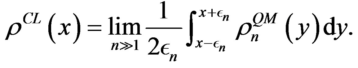
It is well known that the classical and quantum probability density functions for periodic systems approach each other in a locally averaged sense when the principal quantum number becomes large, i.e.
 (1)
(1)
Note that  is directly related with the standard deviation
 , so that
  decreases when increasing
 . Equation (1) can be computed analytically only for extremely simple systems, such as the infinite square well potential [10]. For more complex systems, like the harmonic oscillator and the Kepler problem, the associated integral are more complicated.
In our previous paper we introduced a mathematical procedure to derive the classical limit of quantum probability distributions. We write the classical and quantum distributions as a Fourier expansion, i.e.
 (2)
(2)
where  and
and  are the Fourier coefficients of each expansion respectively. Substituting (2) into (1), we find that the Fourier coefficients have a similar behavior for large quantum number
 :
:
 (3)
(3)
 -dependent corrections may arise in Equation (3) because we do not consider the limit on
 . This implies that even at a macroscopic level
  remains finite, i.e. Heisenberg’s theorem is still valid. We represent an alternative evaluation of Equation (1).
3. The Classical Limit
According to Newtonian physics, the trajectories for bound state motion  of a particle in the Coulomb field
  are ellipses with parametric equation:
 (4)
(4)
where  is the semimajor axis and
the eccentricity [14]. Then the classical radial probability density (CRPD) is given by:
 (5)
(5)
which is defined for , with
 . It can be shown that Equation (5) is properly normalized.
On the other hand, the solutions for the quantummechanical Kepler problem are well known, i.e.  , where
  are the radial wave functions of the Schrödinger equation and
  are the spherical harmonics [2,15]. Then the normalized quantum radial probability density (QRPD) is given by
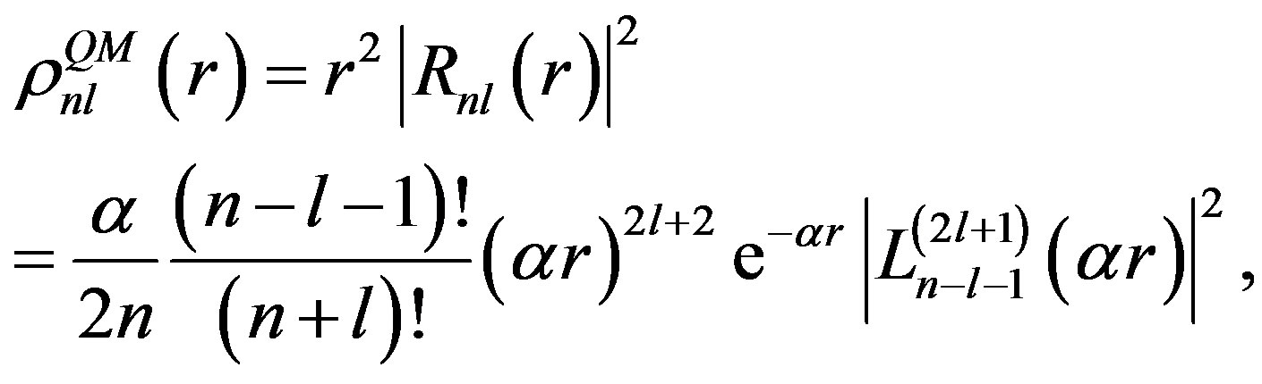 (6)
(6)
where  (where
  is the Bohr’s radius) and
 is an associate Laguerre polynomial. The angular distribution
  is properly normalized.
Now we study the conditions under which the quantum distribution leads to its classical analogue. The angular behavior can be explored directly. It is apparent that when  has its maximum value,
  , the angular distribution reduces to
 , which becomes arbitrarily sharp around
  in the limit
 . So, the QRPD will be confined to this plane when
 , like in the classical model. On the other hand, the emergence of
  from
from  is not evident. The relative fluctuation expectation values in the radial variable, calculated in the atomic state
  are
are
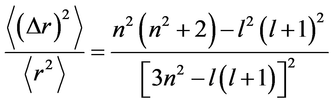 (7)
(7)
[15]. We observe that this fluctuation vanishes like  when
when  has its maximum value,
 . Thus we see that in the limit
  the radial probability distribution of the atomic state
  approximates an equatorial circular orbit. In the opposite case, when
  has its minimum value,
  , we see that the radial probability distribution is broad and corresponds to narrow ellipses that have degenerated into straight lines through the center of the orbit. Therefore, in accordance with Bohr’s correspondence principle, the CRPD emerges from the QRPD when
  becomes large while
  remains fixed.
In Figure 1, the radial probability distribution (Equation (6)) is plotted and, for comparison, we also display the classical distribution (Equation (5)). The turning points are, of course, determined by equating the classical and quantum expressions for the energy and angular momentum, i.e.
 (8)
(8)
respectively [14,15]. The absence of any reasonable similarity is very striking in Figure 1(a). This is, of course, because at low energy the behavior in the quantum regime is very different. On the other hand, in Figures 1(b) and (c) we see that the distributions approach each other in a locally averaged sense as  increases while
  remains fiexed. Although these results seem pretty, it has not been shown with any other procedure.
Next we concentrate on the calculation of the classical limit. We first we calculate the Fourier coefficients. The associated integral is rather involved but fortunatetly it
 (a)
(a) (b)
(b)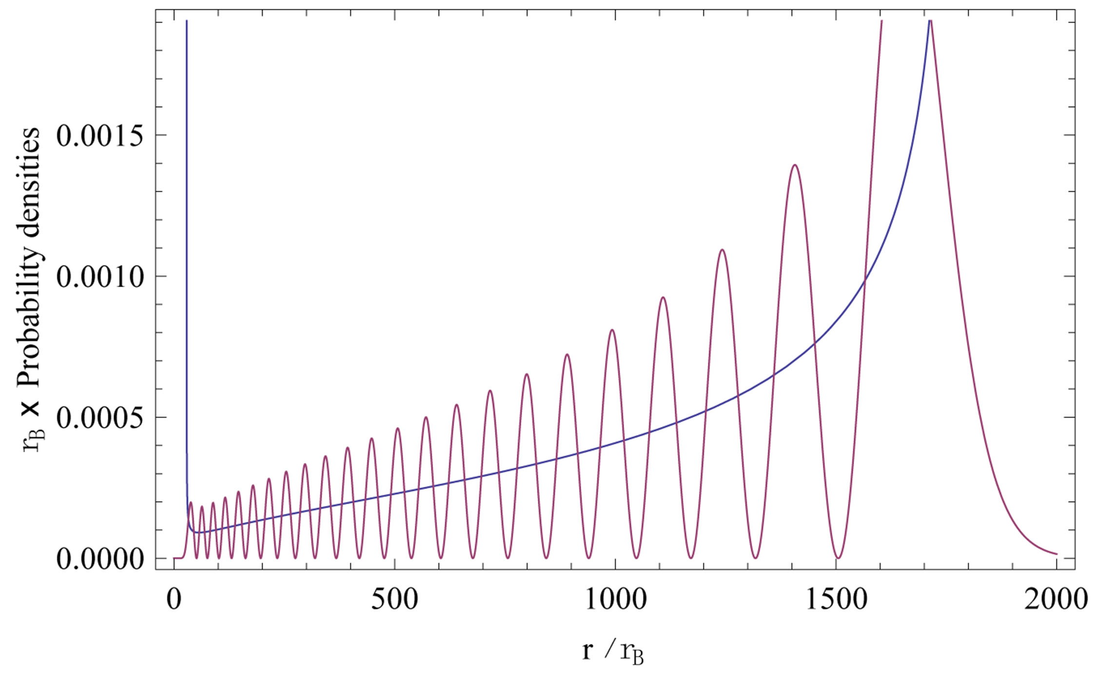 (c)
(c)
Figure 1. Comparison of the quantum radial probability density (red line) along with the classical radial probability density (blue line). Frame (a) shows the QRPD for the ground state along with the CRPD. Frames (b) and (c) show the QRPD for  with
with  and
and  with
with  stationary states along with the CRPD, respectively.
has been reported in Ref. [16], i.e.
 (9)
(9)
where  and
and  denotes the second Appell hypergeometric function. The asymptotic behavior of the above equation is not reported in the literature, but we now explore some special cases.
The simplest case results for the maximum angular momentum. We first we observe that Equation (9) reduces to  when
when . On the other hand, from equation (8) we find that
 , so that the asymptotic behavior of the Fourier coefficients
  for
for  large becomes
 (10)
(10)
Thus the inverse Fourier transform gives a Dirac’s delta function located at , i.e.
 (11)
(11)
which is the classical result for a circular orbit. Note that Equation (8) implies that the eccentricity  tends to zero as
  becomes infinite, so that the semimajor axis
  equals the semiminor axis and coincides with the radius of the circular orbit. This particular result illustrates in a clear fashion the applicability of the simple mathematical formulation of the correspondence principle given in Ref. [13].
The next case we consider is for large angular momentum, i.e. . We observe that the second Appell hypergeometric function
  appearing in Equation (9) can be approximated by a Gauss hypergeometric function
  for
for  large [17,18], so we find
 (12)
(12)
where . Note that Equation (12) is a polynomial function of order
 . In order to study the asymptotic behavior of the Equation (12), we first rewrite it conveniently as a polynomial series, i.e.
 (13)
(13)
The problem is now reduced to computing the asymptotics of the coefficients appearing in the summation. In the limiting case that we have considered,  with
with  remaining fixed, a first approximation of Equation (13) gives
 (14)
(14)
where  and
and  are the Bessel functions of the first kind. We point out that we can calulate higher order approximations, but for our purposes we consider here only the first one.
The inverse Fourier transform of Equation (14) which can be found in Ref.[19] gives
 (15)
(15)
which corresponds exactly with the classical radial probability density. The higher order corrections involve a series depending on successive powers of .
.
4. Discussion
When a theory succeeds in describing physical reality in a better way then its predecessor, as is the case of relativity compared with Newton’s theory, and both share an essential physical framework, a purely mathematical reduction of the more general theory to the restricted one is generally possible. Even in the case of the special theory of relativity, Bacry and Levy-Leblond [20] have shown that the low velocity limit of Lorentz transformations for space-like intervals  display nonGalilean features, as the time-ordering of two such independent events may be reversed for some observers. The quantum-classical relation is more subtle, given that the conceptual frameworks of these theories are fundamentally different. The question that naturally arises is the way in which quantum theory reduces to classical theory when applied to a macroscopic system. Zurek, for example, studies the role that the enviroment has on producing the effect of decoherence [21].
In the classical regime, the probability distribution  becomes entirely confined between two turning points and as
  is kept constant, momentum is also confined within a finite interval. Such a state is no longer describable by a wave function [22]. The quantum-mechanical case is radically different. On the one hand, the probability distribution
  is distributed in all space, so the probability that the particle is in the volume
  is given by
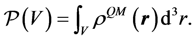 (16)
(16)
On the other hand, it is impossible to define quantum turning points (as in the classical sense) because of Heisenberg’s theorem works. These facts make these theories seem conceptually incompatible.
It is well known, however, that the probability distributions,  and
and , approach each other in a locally averaged sense, when some appropriate quantum numbers become large [9-11]. Although this result seems simple, there is no simple mathematical procedure to prove this assertion. In a previous work [13], we introduced a mathematical procedure to prove that the quantum probability distribution leads to the classical one when applied to the high energy regime. Our method is based on both the Bohr’s correspondence principle and the local averages of the quantum probability distribution. Note that we do not need to consider the limit where
 . There exist higher order corrections which can be expressed as powers of
 . The classical result for the probability distribution is recovered as the
  -independent zeroth order term. In this approach Heisenberg’s theorem applies even at the macroscopic level. This is philosophically more satisfactory than actually using the
  limit and provides corrections that are associated in principle with the classical-quantum borderline.
As can be seen from Figure 1 and other cases like the harmonic oscillator, as the principal quantum number is increased,  becomes spatially confined in a couple of points, then becomes a rapidly oscillatory function inside this region while the outside is strongly suppressed. We therefore observe macroscopically a motion bounded by this couple of points, identified as the classical turning points and the probability of finding the particle outside this region, i.e. Equation (16), tends to zero as the energy increases, so that it becomes forbidden in this regime. When we use our procedure, the oscillatory behavior of the quantum distribution is averaged out and becomes a smooth function in the macroscopically accessible region. The function cancels outside this region and the turning points look like infinite walls, akin to the macroscopic behavior.
5. Conclusions
Since the birth of quantum mechanics, prevails the belief that is the general theory, and that classical mechanics must be deducible from it; however there is not a satisfactory demonstration of this belief. The answer to that question took the form of the heuristic principle, known as the correspondence principle. Although the importance of correspondence principle is largely undisputed, there is far less agreement concerning how it should be defined. The approaches discussed in almost all textbooks (as WKB approximation and Ehrenfest’s theorem) are not generally valid. No doubt that the classical limit is not a simple problem.
In a previous paper we introduced a simple procedure to connect the classical and quantum probability distributions for the harmonic oscillator case and we argue its general validity. We now report analytical results for the Kepler problem. It is noteworthy that these results cannot be achieved by any other procedure. The main result of this paper is the emergence of semi-classical Bohr’s circular orbits from purely quantum mechanical data.
We consider our approach demonstrates that quantum mechanics is applicable in every scale of nature, and that the macroscopic world is a consequence of its asymptotic behavior in the high energy regime. Even though our approach gives the correct classical results for periodic quantum systems, it is far from the general solution to the classical limit problem. There are still related open problems needed for a general mathematical formulation of the classical limit problem, as the study of the unbound systems. We are currently exploring residual effects of quantum transitions at macrocopic level [23].
REFERENCES
- A. J. Makowski, European Journal of Physics, Vol. 27, 2006, pp. 1133-1139. doi:10.1088/0143-0807/27/5/012
- L. E. Ballentine, “Quantum Mechanics: A Modern Development,” World Scientific, New York, 1998.
- L. E. Ballentine, Y. M. Yang and J. P. Zibin, Physical Review A, Vol. 50, 1994, pp. 2854-2859. doi:10.1103/PhysRevA.50.2854
- M. Berry, Physica Scripta, Vol. 40, 1989, pp. 335-336. doi:10.1088/0031-8949/40/3/013
- L. S. Brown, American Journal of Physics, Vol. 40, 1972, pp. 371-376. doi:10.1119/1.1986554
- L. S. Brown, American Journal of Physics, Vol. 41, 1973, pp. 525-530. doi:10.1119/1.1987282
- D. Bhaumik, B. Dutta-Roy and G. Ghosh, Journal of Physics A: Mathematical and General, Vol. 19, 1986, pp. 1355-1364. doi:10.1088/0305-4470/19/8/017
- S. Nandi and C. S. Shastry, Journal of Physics A: Mathematical and General, Vol. 22, 1989, pp. 1005-1016. doi:10.1088/0305-4470/22/8/016
- G. Yoder, American Journal of Physics, Vol. 74, 2006, p. 404. doi:10.1119/1.2173280
- R. W. Robinett, American Journal of Physics, Vol. 63, 1995, pp. 823-832. doi:10.1119/1.17807
- E. G. P. Rowe, European Journal of Physics, Vol. 8, 1987, pp. 81-87. doi:10.1088/0143-0807/8/2/002
- A. R. Edmonds, “Angular Momentum in Quantum Mechanics,” Princeton University Press, Princeton, 1974.
- J. Bernal, A. Martn-Ruiz and J. Garca-Melgarejo, Journal of Modern Physics, Vol. 4, 2013, pp. 108-112. doi:10.4236/jmp.2013.41017
- H. Goldstein, C. P. Poole and J. P. Safko, “Classical Mechanics,” Addison-Wesley, San Francisco, 2002.
- R. Liboff, “Introductory Quantum Mechanics,” 4th Edition, Addison-Wesley, Boston, 2002.
- H. M. Srivastava, H. A. Mavromatis and R. S. Alassar, Applied Mathematics Letters, Vol. 16, 2003, pp. 1131- 1136. doi:10.1016/S0893-9659(03)90106-6
- A. P. Prudnikov, Yu. A. Brychkov and O. I. Marichev, “Integrals and Series, Vol. 3: More Special Functions,” Gordon and Breach Science Publishers, New York, 1989.
- L. J. Slater, “Generalized Hypergeometric Functions,” Cambridge University Press, Cambridge, 2008.
- M. Abramowitz and I. Stegun, “Handbook of Mathematical Functions: with Formulas, Graphs, and Mathematical Tables,” Dover Publications, New York, 1965.
- H. Bacry and I.-M. Lavy-Leblond, Journal of Mathematical Physics, Vol. 9, 1968, pp. 1605-1615. doi:10.1063/1.1664490
- W. H. Zurek, Reviews of Modern Physics, Vol. 75, 2003, pp. 715-775. doi:10.1103/RevModPhys.75.715
- D. Sen and S. Sengupta, Indian Journal of Physics, Vol. 73, 1999, pp. 135-139.
- A. Martín-Ruiz, J. Bernal and A. Carbajal-Dominguez, “Residual Effects of Quantum Transitions at Macroscopic Level,” in Press.