

Applied Mathematics
Vol.06 No.02(2015), Article ID:54040,20 pages
10.4236/am.2015.62036
The Barone-Adesi Whaley Formula to Price American Options Revisited
Lorella Fatone1, Francesca Mariani2, Maria Cristina Recchioni3, Francesco Zirilli4
1Dipartimento di Matematica e Informatica, Università di Camerino, Camerino, Italy
2Dipartimento di Scienze Economiche, Università degli Studi di Verona, Verona, Italy
3Dipartimento di Management, Università Politecnica delle Marche, Ancona, Italy
4Dipartimento di Matematica “G. Castelnuovo”, Università di Roma “La Sapienza”, Roma, Italy
Email: lorella.fatone@unicam.it, francesca.mariani@univr.it, m.c.recchioni@univpm.it, zirilli@mat.uniroma1.it
Copyright © 2015 by authors and Scientific Research Publishing Inc.
This work is licensed under the Creative Commons Attribution International License (CC BY).
http://creativecommons.org/licenses/by/4.0/



Received 22 January 2015; accepted 10 February 2015; published 13 February 2015
ABSTRACT
This paper presents a method to solve the American option pricing problem in the Black Scholes framework that generalizes the Barone-Adesi, Whaley method [1] . An auxiliary parameter is introduced in the American option pricing problem. Power series expansions in this parameter of the option price and of the corresponding free boundary are derived. These series expansions have the Baroni-Adesi, Whaley solution of the American option pricing problem as zero-th order term. The coefficients of the option price series are explicit formulae. The partial sums of the free boundary series are determined solving numerically nonlinear equations that depend from the time variable as a parameter. Numerical experiments suggest that the series expansions derived are convergent. The evaluation of the truncated series expansions on a grid of values of the independent variables is easily parallelizable. The cost of computing the n-th order truncated series expansions is approximately proportional to n as n goes to infinity. The results obtained on a set of test problems with the first and second order approximations deduced from the previous series expansions outperform in accuracy and/or in computational cost the results obtained with several alternative methods to solve the American option pricing problem [1] -[3] . For example when we consider options with maturity time between three and ten years and positive cost of carrying parameter (i.e. when the continuous dividend yield is smaller than the risk free interest rate) the second order approximation of the free boundary obtained truncating the series expansions improves substantially the Barone-Adesi, Whaley free boundary [1] . The website: http://www.econ.univpm.it/recchioni/finance/w20 contains material including animations, an interactive application and an app that helps the understanding of the paper. A general reference to the work of the authors and of their coauthors in mathematical finance is the website: http://www.econ.univpm.it/recchioni/finance.
Keywords:
American Option Pricing, Perturbation Expansion

1. Introduction
American call and put options are one of the most traded products in financial markets. They are traded either standing alone or embedded in a variety of financial contracts such as, for example, convertible bonds, mortgages or life insurance policies. The fast and accurate evaluation of American option prices and of the corresponding free boundaries is an important problem in mathematical finance. Let us restrict our attention to the American option pricing problem in the Black Scholes framework. Many methods have been suggested to solve this problem. In particular several hybrid methods have been suggested. These methods combine analytical and numerical approximations. For example let us mention the hybrid methods proposed by Geske, Johnson (1984) [4] , Barone-Adesi, Whaley (1987) [1] , Kim (1990) [5] , Bunch, Johnson, (1992) [6] , Bjerksund, Stensland (1993) [7] , Ju, Zhong (1999) [2] , Barone-Adesi (2005) [8] and Zhu (2006) [9] .
In [1] Barone-Adesi and Whaley write the American option price as the sum of the price of the corresponding European option and of a quantity called early exercise premium. The European option price is given by the Black Scholes formula and the early exercise premium is approximated with the solution of a free boundary value problem for an ordinary differential equation. This ordinary differential equation is obtained dropping the time derivative term in the partial differential equation satisfied by the early exercise premium. Barone-Adesi and Whaley [1] give a simple formula for the solution of this free boundary value problem for an ordinary differential equation. Moreover they determine an approximation of the free boundary solving numerically a nonlinear equation that depends from the time variable as a parameter. This approximate solution of the American option pricing problem is called Barone-Adesi, Whaley formula and is widely used in the financial markets by practitioners. An exhaustive review of the methods used to solve the American option pricing problem and of the developments of the Barone-Adesi, Whaley method during the period 1987-2005 can be found in Barone- Adesi (2005) [8] . For example in 1999 Ju, Zhong [2] reconsidered the Barone-Adesi, Whaley formula of the early exercise premium. The Ju, Zhong formula [2] introduces a correction to the Barone-Adesi, Whaley approximation of the early exercise premium. This correction consists in writing the early exercise premium as the product of the Barone-Adesi, Whaley early exercise premium times a time-independent function determined solving an ordinary differential equation. When long dated options are considered, the Ju, Zhong formula improves the approximate option price obtained with the Barone-Adesi, Whaley formula.
Given a positive integer n, Geske and Johnson [4] approximate the price of an American put option using an n-fold compound option. They assume that exercise decisions are taken only at some known time values. These time values are a set of n points. In [4] Geske and Johnson deduce a formula to approximate the American put option price with a piecewise solution of the Black Scholes partial differential equation subject to boundary conditions imposed at the decision times. Moreover, using Richardson extrapolation, they show how to approximate the Geske, Johnson formula with a simple polynomial expression. Bunch and Johnson [6] refine the results obtained in [4] determining the n exercise times that maximize the accuracy of the option prices obtained.
In [7] Bjerksund and Stensland approximate the solution of the American option pricing problem assuming a flat early exercise boundary and using a trigger price. Bjerksund and Stensland reduce the evaluation of an American call option with exercise price E and maturity time T to the evaluation of a European call up-and-out barrier option with knock-out barrier X, strike price E and maturity time T. A rebate given by
 is received by the holder of the option at the knock-out time when the option is exercised prior to maturity time. The barrier X is the flat boundary that approximates the free boundary of the American option pricing problem. In [7] the problem of choosing X is studied. In [10] the approximation of the free boundary used in [7] is refined. In fact in [10] the time interval where the problem is studied is divided in two disjoint subintervals and a flat early exercise boundary is used in each subinterval.
Zhu (2006) [9] considers the American put option pricing problem and derives an explicit formula of the American put option price associated to a numerically approximated free boundary. This formula is a Taylor’s series expansion with infinitely many terms. Each term of this Taylor’s expansion considered contains several integrals that must be evaluated numerically. In [11] I. J. Kim, Jang, K. T. Kim show that the numerical evaluation of Zhu’s formula is cumbersome and suggest a method to approximate the free boundary of the American option pricing problem. This method consists in the numerical solution of the integral equation satisfied by the free boundary deduced in [3] by Little, Pant, Hou. The solution of the American put option pricing problem suggested in [11] combines the integral formula of the option price obtained by I. J. Kim [5] with the approximation of the corresponding free boundary obtained solving numerically the integral equation presented in [3] . Note that in the option price formula contained in [5] there are several integrals that must be evaluated numerically.
To solve the American option pricing problem instead of using hybrid methods it is possible to use only numerical methods. For example the finite differences method (see [12] ), the Monte Carlo method (see [13] -[18] ), and the regression method (see [19] [20] ) can be used to solve the American option pricing problem.
Usually hybrid methods are computationally cheaper than numerical methods. However in many circumstances numerical methods provide approximate solutions of the American option pricing problem that are more accurate than those obtained with hybrid methods. In fact, at least in principle, the solutions provided by numerical methods can be made arbitrarily accurate choosing appropriately the values of the parameters that define the approximation computed. Instead many hybrid methods have a certain accuracy that depends from the problem under consideration and this accuracy cannot be changed choosing parameter values. That is most of the solutions found with hybrid methods do not converge to the exact solution of the American option pricing problem when a suitable limit is taken. Moreover most hybrid methods give satisfactory results when pricing problems with short maturity times are considered. The results obtained with these methods deteriorate when problems with medium or long maturity times are considered.
This paper presents a hybrid method to solve the American option pricing problem. We introduce an auxiliary parameter in the American option pricing problem and we deduce power series expansions in this parameter of the option price and of the corresponding free boundary. Explicit formulae (depending from the free boundary) are given for the coefficients of the option price series. The partial sums of the free boundary series are determined solving numerically nonlinear equations that depend from the time variable as a parameter. These series expansions are a formal solution of the American option pricing problem. Numerical experiments suggest that the series obtained are convergent. The zero-th order term of the series expansions is the Barone-Adesi, Whaley solution of the American option pricing problem [1] (i.e. the Barone-Adesi, Whaley formula). The first order approximation of the option price deduced from the expansions developed here has some similarities with the early exercise premium formula suggested by Ju, Zhong [2] .
Test problems taken from [1] [2] and [3] are studied. The behaviour of the truncated series expansions on these test problems is studied. In particular in the numerical experiments presented we use the n-th order approximate solutions deduced from the expansions when n = 0, 1, 2 to solve the test problems considered. These experiments show that each approximation order of the solution deduced from the expansions adds roughly one correct significant digit to the results obtained. Moreover for n = 0, 1, ∙∙∙ the computation of the n-th order approximation deduced from the expansions of the solution of the American option pricing problem on a grid of values of the independent variables is easily parallelizable and its computational cost is “substantially” linear in n as n goes to infinity. In particular the numerical experiments show that when we consider options with intermediate maturity times (i.e.: maturity times ranging in the interval 3 - 10 years) the first and the second order approximations of the solution obtained from the series expansions improve substantially the approximate solution obtained using the Barone-Adesi, Whaley formula (see in Section 4, Table 1, Table 3, Table 4 and Figure 2). For example the improvement obtained with the higher order terms of the expansions is significant when we compare the approximations of the free boundary of the American option pricing problem obtained using the Barone-Adesi, Whaley formula with those obtained using the n-th order truncated power series expansions, n = 1, 2 (see Section 4, Table 1, Table 4 and Figure 2). Note that the Barone-Adesi, Whaley formula gives excellent results when we consider options with short or with long maturity times and that in these circumstances there is no room for improvements of practical value (see [1] ).
The website: http://www.econ.univpm.it/recchioni/finance/w20 contains material including animations, an interactive application and an app that helps the understanding of the paper. More general references to the work of the authors and of their coauthors in mathematical finance are available in the website: http://www.econ.univpm.it/recchioni/finance.
The paper is organized as follows. In Section 2 we formulate the American call option pricing problem in the Black Scholes framework and we introduce the auxiliary parameter that is used to solve it. In Section 3 we deduce the perturbation expansions in this auxiliary parameter of the American call option price and of the corresponding free boundary. The analysis of Sections 2 and 3 can be easily extended from the case of the American call option pricing problem to the case of the American put option pricing problem. This extension is omitted for simplicity. In Section 4 we present the results obtained with the method developed in Sections 2 and 3 on a set of test problems involving American call and put options. These results are compared with those discussed in the scientific literature obtained with some alternative methods to solve the American option pricing problem.
2. The American Option Pricing Problem in the Black Scholes Framework
We follow Barone-Adesi and Whaley [1] and we consider the problem of pricing American call and put options on commodities in the Black Scholes framework.
Let t be a real variable that denotes time and St, t > 0, be a real stochastic process that models the commodity price, that is for t > 0 the random variable St represents the commodity price at time t. We assume that under the risk neutral measure the commodity price satisfies the following stochastic differential equation:
 (1)
(1)
where b,
 are real parameters, zt, t > 0, is the standard Wiener process such that
 and dzt is its stochastic differential. Equation (1) is known as Black Scholes asset price equation. The parameter
 is the volatility or instantaneous standard deviation and b is the cost of carrying parameter. In the most common situations we have
 where r > 0 is the risk free interest rate and d > 0 is the continuous dividend yield, see [1] . When needed Equation (1) is equipped with an initial condition.
To keep the exposition simple we study only the American call option pricing problem. The American put option pricing problem can be studied analogously. However in the test problems presented in Section 4 the method developed here to solve the American option pricing problem is used to evaluate both call and put options.
Let t = 0 be the current time, consider the problem of pricing an American call option having exercise price E > 0 and maturity time T > 0 written on a commodity whose price St, t > 0, satisfies (1). The price ,
,
 ,
,
 , of this option and the corresponding free boundary
 ,
,
 , solve the following problem [21] :
 (2)
(2)
with boundary conditions:
 (3)
(3)
 (4)
(4)
 (5)
(5)
and final condition:
 (6)
(6)
Problem (2), (3), (4), (5), (6) is the American call option pricing problem in the Black Scholes framework. It is a free boundary value problem for the partial differential Equation (2) whose unknowns are: the option price ,
,
 ,
,
 , and the free boundary
 ,
,
 , see [22] . Note that the boundary condition (3) can be omitted. In fact condition (3) follows from the degeneracy in
 of (2) and from the fact that in mathematical finance only bounded solutions of (2) are meaningful (see [21] Chapter 3, p. 48-49). However to make easier the understanding of some choices made later (see Section 3) we prefer to state (3) explicitly.
Let us consider the change of variable: ,
,
 , the variable
 is called time to maturity, and let us define:
 ,
,
 ,
,
 ,
,
 ,
, . Problem (2), (3), (4), (5), (6) rewritten in the variables S,
 for the unknowns CA, S* becomes:
 (7)
(7)
with boundary conditions:
 (8)
(8)
 (9)
(9)
 (10)
(10)
and initial condition:
 (11)
(11)
Let ,
,
 ,
,
 , be the Black Scholes price of the European call option having strike price E, maturity time T and parameters r, b,
 . The price
 ,
,
 ,
,
 , has a simple expression given by the Black Scholes formula [21] . Note that CE is defined for
 ,
, . As done in [1] we seek a solution of problem (7), (8), (9), (10), (11) given by the sum of
 ,
,
 ,
,
 , and of a quantity called early exercise premium denoted with
 ,
,
 ,
, . That is we assume that:
 (12)
(12)
Substituting (12) in (7), (8), (9), (10), (11) and using the fact that CE satisfies the Black Scholes partial differential Equation (7), the boundary condition (8) and the initial condition (11) we obtain the following problem:
 (13)
(13)
with boundary conditions:
 (14)
(14)
 (15)
(15)
 (16)
(16)
and initial condition:
 (17)
(17)
Problem (13), (14), (15), (16), (17) is a free boundary value problem for the partial differential Equation (13) in the unknowns ,
,
 ,
,
 , and
, and ,
, .
.
We assume that the early exercise premium e has the following form (see [1] ):
 (18)
(18)
where ,
,
 , is a sufficiently regular function that will be chosen later and
 ,
,
 ,
,
 , is an auxiliary unknown that must be determined solving (13), (14), (15), (16), (17), (18). Substituting (18) in (13) we have:
 (19)
(19)
where
 and
and . Choosing
 ,
,
 , (see [1] ), Equation (19) becomes:
 (20)
(20)
Equation (18) and the previous choice of K imply that the boundary conditions (14), (15), (16) can be rewritten respectively as:
 (21)
(21)
 (22)
(22)
 (23)
(23)
Note that in the formulation of problem (20), (21), (22), (23) we use the two variables
 and K, and recall that these two variables are linked by the condition
 ,
, . Moreover from the choice
 ,
,
 , it follows that
 . This implies that when the function f is well behaved in
 the function e defined in (18) satisfies the initial condition (17).
In [1] Barone-Adesi and Whaley dropped the term
 in Equation (20) and solved the problem that remains. This is an ingenious and fruitful idea. In fact after dropping the term
 in (20) the problem that remains is easy to solve, see [1] , moreover the term dropped tends to zero when
 goes to zero and when
 goes to T and T goes to infinity. Let f0,
 be the solution of the problem obtained from (20), (21), (22), (23) dropping the term
 in (20) determined by Barone-Adesi and Whaley in [1] . The function f0 has a closed form expression that contains the free boundary
 ,
, . The free boundary
 is defined implicitly as solution of the nonlinear Equation (23) when we have
 ,
, . The approximation of the free boundary of Barone-Adesi and Whaley [1] is obtained solving numerically the nonlinear equation (23) when
 ,
, . Note that the nonlinear Equation (23) that defines
 depends from f0. The approximate solution of the American option pricing problem given by the functions f0,
 is called Barone-Adesi, Whaley formula. With abuse of notation in this paper
 ,
,
 , denotes both the Barone-Adesi, Whaley free boundary defined implicitly by the nonlinear equation (23) when
 ,
,
 , and its numerical approximation.
In problem (20), (21), (22), (23) we introduce a real parameter ,
, . The parameter
 is the auxiliary parameter mentioned in the introduction that is used to solve the American call option pricing problem. That is instead of problem (20), (21), (22), (23) we consider problem:
 (24)
(24)
 (25)
(25)
 (26)
(26)
 (27)
(27)
in the unknowns ,
,
 ,
, . The initial condition (17) and Equation (18) rewritten for the functions
 ,
,
 become respectively:
 (28)
(28)
and
 (29)
(29)
Note that when
 Equation (24) reduces to Equation (20), that is when
 problem (24), (25), (26), (27), (28), (29) reduces to the American call option pricing problem (20), (21), (22), (23), (17), (18). Moreover when
 problem (24), (25), (26), (27) reduces to the problem obtained from (20), (21), (22), (23) dropping
the term
 in (20), that is when
 problem (24), (25), (26), (27) reduces to the problem con-
sidered by Barone-Adesi and Whaley in [1] . Note that the solution determined in [1] of (24), (25), (26), (27) when
 satisfies the conditions (28), (29) with
 .
.
Moreover problem (24), (25), (26), (27), (28), (29) when
 is a singular perturbation problem. In fact when
 in Equation (24) the term containing the higher order derivative with respect to K is multiplied by zero. This fact suggests that when
 an expansion of
 ,
,
 in powers of
 with base point
 cannot hold uniformly in K and S when
 ,
,
 ,
,
 , due to the presence of a boundary layer in K = 0. In singular perturbation theory this kind of problems is approached using the method of matched asymptotic expansions [23] . The matched asymptotic expansion method builds a uniform approximation of the solution of problem (24), (25), (26), (27), (28), (29) when
 ,
,
 ,
,
 , and
, and
 matching two series (called inner and outer expansions). Let
 be the Landau symbol, roughly speaking in the K variable the inner expansion of the option price holds when
 ,
,
 ,
,
 , and the outer expansion of the option price holds when
 ,
,
 ,
,
 , and only the matched expansion holds uniformly in the entire solution domain (see [23] for further details). However it is important to point out that in problem (24), (25), (26), (27), (28), (29)
 is not a parameter of the model,
 is only an auxiliary parameter added to the model and that in finance only the solution of the previous problem when
 is meaningful. The behaviour of the solution of problem (24), (25), (26), (27), (28), (29) when
 is of no interest in finance. This observation suggests that in the solution of the problem (24), (25), (26), (27), (28), (29) it should be possible to avoid the study of the boundary layer in K = 0 that appears when
 . That is it should be possible to solve problem (24), (25), (26), (27), (28), (29) when
 with an ad hoc procedure avoiding the matched asymptotic expansions of singular perturbation theory needed to study the problem when
 . In fact in Section 3 we build a kind of outer series expansion of the solution of problem (24), (25), (26), (27), (28), (29). More specifically in Section 3 we neglect the initial condition (28) and we impose Equation (24) and the boundary conditions (25), (26), (27) in
 order by order in perturbation theory to a series expansion of the solution of problem (4), (25), (26), (27), (28), (29). This procedure is a straightforward generalization of the procedure followed by Barone-Adesi and Whaley in [1] to solve problem (24), (25), (26), (27), (28), (29) when
 .
.
The zero-th order term of the expansions in powers of
 of
of ,
,
 obtained in Section 3 when
 are the functions f0,
 determined by Barone-Adesi and Whaley in [1] . Moreover the expansions developed in Section 3 rewritten in the variables S,
 evaluated in
 and (29) are a formal series expansion of the solution of the American option pricing problem (13), (14), (15), (16), (17).
Let us recall that in [24] a similar approach has been used in the study of barrier options. In fact in [24] it is considered the problem of pricing (put up-and-out) barrier options with time-dependent parameters in the Black Scholes framework. An auxiliary parameter is introduced in the barrier option pricing problem and a perturbation expansion in this parameter of the barrier option price is deduced. Note that the perturbation problem studied in [24] is a regular perturbation problem, while the perturbation problem considered here when
 is a singular perturbation problem.
3. A Series Expansion of the Solution of the American Option Pricing Problem
Let us drop the initial condition (28) from problem (24), (25), (26), (27), (28), (29). That is let us consider the equation:
 (30)
(30)
with the boundary conditions:
 (31)
(31)
 (32)
(32)
 (33)
(33)
Recall that once determined ,
,
 as solution of (30), (31), (32), (33) we will recover the function e using (29) and that when
 is well behaved in
 the function e determined in this way will satisfy the initial condition (28) as a consequence of the choice
 ,
,
 , that implies
 . Let us assume that the following expansions in powers of
 of the functions
 ,
,
 ,
,
 , hold:
 (34)
(34)
 (35)
(35)
where the functions ,
,
 ,
,
 are independent of
 .
.
For later convenience we define the partial sums ,
,
 ,
,
 ,
,
 , of the series (34), (35), that is:
 (36)
(36)
 (37)
(37)
Note that for
 the problems that follow define the function
 for
for ,
, . To give a meaning to the sums contained in (34) and (36) we extend with zero the function
 when
when ,
,
 ,
, . With abuse of notation
 denotes both the original function and the extended function
 .
.
We impose (30), (31), (32), (33) to the series expansions (34), (35), order by order in powers of . For n = 0, 1, ∙∙∙ the unknowns of the n-th order problem are the functions
 ,
, . Note that as unknown of the n-th order problem, we use
 instead of
 , n = 0, 1, ∙∙∙. This is due to the fact that since we are interested only in the solution of problem (30), (31), (32), (33) when
 we impose the boundary conditions (32), (33) in
 instead of imposing them in
 . This is what has been done by Barone-Adesi and Whaley [1] in the solution of the zero-th order problem. We simply extend the idea of Barone-Adesi and Whaley from the zero-th order problem to the n-th order problem, n = 1, 2, ∙∙∙. Proceeding in this way we obtain:
For n = 0 the zero-th order problem is:
 (38)
(38)
with boundary conditions:
 (39)
(39)
 (40)
(40)
 (41)
(41)
for n = 1, 2, ∙∙∙ the n-th order problem is:
 (42)
(42)
with boundary conditions:
 (43)
(43)
 (44)
(44)
 (45)
(45)
The problems (38), (39), (40), (41) and (42), (43), (44), (45) are respectively free boundary value problems for the ordinary differential Equations (38) and (42). These problems depend from the parameter ,
, . The boundary conditions (40), (41) and (44), (45) are the boundary conditions imposed in
 derived from (32), (33). Note that we have:
 ,
,
 where f0,
 is the Barone-Adesi, Whaley solution of the American option pricing problem deduced in [1] . Numerical experiments have shown that the approximations of the first few orders of f and
 deduced from the series expansions (34), (35) with the boundary conditions (40), (41) and (44), (45) imposed to the partial sums (37) evaluated in
 are of higher quality than the corresponding approximations of the same order in
 obtained imposing the boundary conditions (32), (33) order by order in powers of
 in
in . In particular these numerical experiments show that the approximations of
 ,
,
 , obtained solving problem (42), (43), (44), (45) are more accurate than the corresponding approximations obtained evaluating in
 the partial sums
 ,
,
 ,
,
 , where
 ,
,
 are the terms obtained imposing in
 the boundary conditions (32), (33) at the first and at the second order in powers of
 .
.
Let us consider the zero-th order problem (38), (39), (40), (41).
From now on instead of using the notation ,
,
 introduced previously we denote the solution of the zero-th order problem (38), (39), (40), (41) with the notation f0,
 . This choice emphasizes the fact that the zero-th order term of the expansions (34), (35) determined solving the previous problems is the Barone-Adesi, Whaley solution of the American option pricing problem. As done in [1] we seek a solution f0 of (38), (39), (40), (41) of the following form:
 (46)
(46)
where in (46) the functions
 and q are auxiliary unknowns that must be determined. Substituting (46) in (38) we have:
 (47)
(47)
Equation (47) is satisfied if we impose that:
 (48)
(48)
the quadratic Equation (48) in the unknown q is easily solved, and one of its solutions is:
 (49)
(49)
From (49) it follows that
 is positive when K is positive. This means that when
 is given by (49) the function
 ,
,
 ,
,
 , given by (46) satisfies (39). The second solution of (48) is negative when
 is positive and must be discarded since the corresponding function f0 given by (46) does not satisfy (39).
Substituting the formulae (46), (49) in the Equations (40), (41) we obtain respectively:
 (50)
(50)
and
 (51)
(51)
For
 Equation (50) defines
 as a function of
 and Equation (51) is a nonlinear equation in the unknown
 that depends from the parameter
 . Given
 this last equation is easily transformed in a fixed point problem and solved numerically using Banach iteration,
 . The approximate solution of (51) determined in this way is substituted in (50) to obtain
 . The zero-th order term f0 given by (46), (49), (50) with the numerical approximation of
 substituted in
 multiplied by K (see (18)) is the Baroni-Adesi, Whaley formula of the early exercise premium (see [1] formula (20)). The numerical approximation of
 obtained solving numerically (51) is the Barone-Adesi, Whaley approximation of the free boundary (see [1] , formula (19)). Note that as already said with abuse of notation in the previous formulae
 ,
,
 , denotes both the unknown of the nonlinear Equation (51) and its numerical approximation. This ambiguity is reflected in the functions
 and f0.
Let
 we seek a solution
 of the n-th order problem (42), (43), (44), (45) of the following form:
 (52)
(52)
where the functions ,
,
 ,
,
 , are auxiliary unknowns that must be determined imposing (42), (43), (44), (45). Substituting formula (52) in Equation (42) it is easy to see that in order to satisfy (42) it is sufficient to impose that the functions
 ,
,
 ,
,
 , satisfy the following systems of linear equations:
 (53)
(53)
 (54)
(54)
 (55)
(55)
To keep the notation simple in (53), (54), (55) we have omitted the dependence from K of the functions ,
,
 ,
, . For
. For
 the unknowns
 ,
,
 , are determined solving the n-th linear system of linear equations contained in (53), (54), (55). In fact for
 the n-th system of linear equations contained in (53), (54), (55) is a system of 2n linear equations in the 2n unknowns
 ,
,
 , that can be solved by backward substitution starting from the n-th Equation (53). Note that due to its special form the computational cost of solving these linear systems obtained in (53), (54), (55) grows linearly in n when n goes to infinity. Finally for
 the coefficient
 and the unknown
 are determined imposing the boundary conditions (44), (45), that is imposing respectively:
 (56)
(56)
and
 (57)
(57)
To keep the notation simple in (56), (57) we have omitted the dependence from
 of
of ,
, . For
. For
 Equation (56) defines
 as a function of
 and of the solution of the n-th linear system contained in (53), (54), (55),
 . Equation (57) is a nonlinear equation in the unknown
 ,
,
 , depending from the parameter
 , that defines implicitly
 ,
,
 ,
, . In the numerical experiments of Section 4 this equation is transformed in a fixed point problem and solved numerically using Banach iteration. The numerical approximation of
 ,
,
 , obtained from the solution of (57) is substituted in (56) and together with the solution of the n-th linear system contained in (53), (54), (55) determines (56). Note that when
 , for simplicity with abuse of notation we denote with
 ,
,
 , both the unknown of (57) and its numerical approximation.
A careful inspection of formulae (46), (51) and (52), (57) shows that for
 the numerical evaluation on a grid of values of the S and
 variables of the n-th order approximations
 ,
,
 of the solution of the American call option pricing problem is easily parallelized.
4. Numerical Results
Let us discuss the numerical results obtained on a set of test problems with the solution method of the American option pricing problem developed in Sections 2 and 3.
We use the trinomial tree method [17] with nT = 1000 time steps to compute the “true value” of the option prices considered in our experiments. The choice nT = 1000 guarantees four correct significant digits in the option prices computed in this Section. The “true value” of the corresponding free boundaries of the American call options considered in our experiments is computed solving numerically the following integral equation (see [25] , [3] and the reference therein):
 (58)
(58)
The free boundary ,
,
 , is the unknown of the integral Equation (58), moreover in (58) the
function
 is the standard normal cumulative distribution and the functions d and
 are given by:
 (59)
(59)
 (60)
(60)
where in (58), (59), (60) T is the maturity time and E is the strike price of the American call option considered. The integral operator contained in (58) is approximated with the composite rectangular rule with time step
 and
and ,
,
 , is approximated on the set of evenly spaced nodes of step
 used to discretize the integral operator. This discretized version of the integral Equation (58) is solved as a fixed point problem using Banach iteration. Let
 denote the integer part of ∙, for
 let
let
 and
and
 be the solution of the discretized version of the integral Equation (58) at the node
 ,
, . For
. For
 let
let
 be the solution of (58) it is easy to see that we have:
 , when
 is fixed. When we consider an American call option and we have
 the algorithm that solves the discretized version of (58) starts from
 choosing
 when
when
 or choosing
 when
when . Recall that when
 (i.e. when the continuous dividend yield d is smaller or equal to zero) in [1] page 307 it is shown that the American call option price reduces to the corresponding European call option price. In fact in this case the free boundary is “at infinity” and the American call option must be exercised at maturity time, that is the value of the early exercise premium is identically zero.
The integral Equation (58) must be modified to deal with American put options (see [3] ). Moreover in the case of put options the algorithm that solves the corresponding discretized integral equation starts from
 choosing
 when
when
 or choosing
 when
when .
.
In the numerical experiments discussed below the discretized versions of Equation (58) for call options and of the analogous equation for put options (see [3] ) are solved iteratively at the points ,
,
 , when
 and
and . That is we consider the unknowns
 ,
,
 ,
,
implicitly defined as solution of the following set of equations (see [25] for further details):
 (61)
(61)
where in the case of call options from Equation (58) we have:
 (62)
(62)
and
 is assigned as specified above. Of course when we consider put options Equation (58) must be substituted with a different integral equation, see [3] , and as a consequence Equation (62) must be modified coherently. Equations (61), (62) (and their analogous for put options) are solved using Banach iteration. For
 and
and
 let
let
 be the j-th element of the sequence generated by Banach iteration applied to (61), (62),
 . The Banach iteration associated to (61) is stopped at the smallest value of the index j that satisfies the condition:
 (63)
(63)
Note that in general the stopping value of the index j defined by (63) depends from ,
, . The “true values” of the option prices and of the corresponding free boundaries defined previously are used as benchmarks to test the approximate solutions of the American option pricing problem computed with the method developed in Sections 2 and 3 and with some alternative methods taken from the scientific literature.
We begin our numerical experiments studying some test problems taken from [1] Section C.4. These test problems consider options on long-term U.S. Treasury bonds (time to maturity up to three years) and long term care insurance inflation options (time to maturity up to ten years and beyond).
In the first experiment we use the values of the Black Scholes parameters of Table V in [1] . That is we consider the following three sets of parameter values: ,
,
 , and
, and , or
, or
 or
or . For each set of Black Scholes parameters we consider three call options with strike price
 and maturity time
 , or
, or , or
, or . The maturity time T is expressed in years.
Table 1 shows several free boundary approximations of the American call option pricing problems specified above when , 5, 10. From left to right Table 1 shows the free boundary
 computed solving iteratively the discretized version of the integral Equation (58) (i.e.
 is the “true free boundary” used as benchmark) and the approximations
 , when
 , discussed in Sections 2 and 3. Recall that
 is the Barone-Adesi Whaley approximation of the free boundary. Table 1 shows that for
 going from the n-th order approximation to
 -th order approximation of the free boundary roughly adds one correct significant digit to the approximation of the free boundary found. This effect is particularly evident when
 , in fact in this case the Barone-Adesi, Whaley approximation of the free boundary is poor and has no correct significant digits. Note that positive values of b correspond to values of the continuous dividend yield
 smaller than the risk free interest rate r. Recall that for American call options when
 and
and
 the integral Equation (58) becomes singular as
 , see [25] .
When
 (i.e. when
 ) Table 2 shows the asset price S, the European call option price CE obtained evaluating the Black Scholes formula, the approximations of the American call option price obtained using the trinomial tree method CT (i.e. CT is the “true value” of the option price used as benchmark), the Barone-Adesi, Whaley option price CBW obtained from (12), (18) when
 ,
,
 and the n-th order approximation
 , derived from (12), (18) and the series expansions presented in Sections 2 and 3 truncated after
 terms,
 . Furthermore Table 2 shows the relative errors:
 and
and ,
, .
.
Table 1 and Table 2 suggest that increasing the approximation order of the solution of the American call option pricing problem that has been deduced from the expansions in powers of
 developed in Sections 2 and 3 (that is increasing n) it is possible to improve substantially the results obtained with the Barone-Adesi, Whaley formula (i.e. the result obtained when
 ).
).
Figure 1 shows the “true” free boundaries of the American call option pricing problem as a function of
 that have been obtained solving numerically the discretized version of the integral Equation (58) when E = 100,
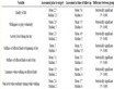
Table 1. Approximations of the free boundary of an American call option with intermediate maturity T and strike price E = 100.

Figure 1. American call option “true” free boundary S* as a function of the time to maturity τ when E = 100, T = 10, r = 0.08, σ = 0.2 and b = −0.04 (solid line , r ≤ r − b), b = 0.0 (dotted line
 , r ≤ r − b), b = 0.04 (dash-dotted line
 , r > r − b).
Table 2. Approximations of the price of an American call option with intermediate maturity T, strike price E = 100 and negative cost of carrying.
T = 10, r = 0.08,
 , and b = −0.04, or b = 0.0, or b = 0.04, and
 . Figure 2 shows the “true” free boundary, the Barone-Adesi, Whaley free boundary, the first and the second order approximations of the free boundary obtained from the expansions of Sections 2 and 3 as a function of the time to maturity
 ,
,
 , when E = 100, T = 10, r = 0.08,
 , b = 0.04. In particular Figure 2 shows that the first order approximation of the free boundary improves significantly the zero-th order approximation of the free boundary (i.e. the Barone-Adesi, Whaley free boundary) and that the second order approximation of the free boundary refines the result obtained with the first order approximation. Figure 3(a) and Figure 3(b) show the “true” and the approximated prices of the American call option corresponding to the free boundaries shown in Figure 2 as a function of the time to maturity
 ,
,
 , T = 10, when the asset price S takes the values S = 90 (Figure 3(a)) and S = 110 (Figure 3(b)). The approximated option prices are obtained using (12), (18) and the zero-th, first and second order approximations of the sum the series expansions developed in Sections 2 and 3. Figure 2 and Figure 3 suggest that the second order corrections of the option price and of the free boundary are necessary to obtain satisfactory approximations of the solution of the American call option pricing problem when we consider

Figure 2. American call option free boundary S* as a function of the time to maturity τ when E = 100, T = 10, r = 0.08, σ = 0.2, b = 0.04: “true” free boundary (solid line), Barone-Adesi, Whaley free boundary (dotted line), first order approximation of the free boundary (dashed line), second order approximation of the free boundary (dash-dotted line).

 (a) (b)
Figure 3. American call option price C as a function of the time to maturity τ for two values of the asset price S = 90 (a), S = 110 (b), when E = 100, T = 10, r = 0.08, σ = 0.2, b = 0.04. “True” price CT (solid line), Barone-Adesi, Whaley price CBW (dotted line), first order approximation
 of the price (dashed line), second order approximation
 of the price (dash-dotted line).
options with intermediate maturity times (i.e. when ) at time t = 0 (i.e.
 ) or at time t close to zero.
Figure 4 shows the American call option price C when
 (i.e. when t = 0), T = 10, E = 100, r = 0.08,
 , b = 0.04 as a function of the asset price S. Note that the option price approximation obtained using the zero-th order term (i.e. the Barone-Adesi, Whaley price) is not accurate (see Figure 4 dotted line). This is a consequence of the fact that the zero-th order approximation of the free boundary is unsatisfactory (see Figure 2, Figure 4). Note that in Figure 4 the payoff function (solid line) is a lower bound for the “true” American call

Figure 4. American call option price C as a function of the asset price S when τ = T = 10, E = 100, r = 0.08, σ = 0.2, b = 0.04. “True” price CT (square-solid line), Barone-Adesi, Whaley price CBW (dotted line), first order approximation
 of the price (dashed line), second order approximation
 of the price (dash-dotted line), and payoff function (solid line). The abscissae of the four marked points show the location of the free boundary: square mark―true free boundary, star mark Barone-Adesi, Whaley free boundary, circle mark―first order approximation of the free boundary, triangle mark― second order approximation of the free boundary.
option price CT and that the first order (dashed line) and the second order (dash-dotted line) approximations obtained using (12), (18) and the series expansions developed in Sections 2 and 3 and the “true” option price CT (square-solid line) overlap while the zero-th order approximation (i.e. the Barone-Adesi, Whaley solution) (dotted line) is not accurate. The abscissae of the four points marked in Figure 4 are the location of the free boundaries: square mark―“true” free boundary, star mark―zero-th order approximation of the free boundary (i.e. Barone-Adesi, Whaley free boundary), circle mark―first order approximation of the free boundary, triangle mark― second order approximation of the free boundary. Note that in Figure 4 the true free boundary and its second order approximation overlap. In Figure 5 we present the relative errors with respect to the “true” option price of the approximated option prices shown in Figure 4 as a function of the asset price. That is Figure 5 shows as a function of the asset price S the relative errors with respect to the “true” option price of the Barone-Adesi, Whaley option price (dotted line), of the first order approximation of the option price (dashed line) and of the second order approximation of the option price (dashed-dotted line) obtained from (12), (18) and the series expansions introduced in Sections 2 and 3. Recall that in Figure 4 and Figure 5 the parameters of the American call option problem considered are: , E = 100, r = 0.08,
 , b = 0.04.
Let us consider the American put option pricing problem. We study a set of test problems similar to those discussed in [2] [3] .
The first test problem involving American put options is taken from Table 5 of [2] and consists in evaluating at time t = 0 the prices of the American put options having E = 100, T = 3 when the underlying asset price ranges from S = 80 to S = 120, that is when ,
,
 , and the Black Scholes parameters have the following values:
 , r = 0.05,
 ,
, .
.
In analogy with the notation introduced previously in the study of the American call option pricing problem we denote with ,
,
 ,
,
 , n = 1, 2, respectively the values of the American put option prices obtained using the trinomial tree method (i.e. the “true value” of the option price used as benchmark), the Barone-Adesi, Whaley formula (for put options) and the n-th order approximation, n = 1, 2, obtained from

Figure 5. Relative errors of the approximations of an American call option price with respect to the “true value” of the price as a function of the asset price S when τ = T = 10, E = 100, r = 0.08, σ = 0.2, b = 0.04: relative error of the Barone-Adesi, Whaley price (dotted line), relative error of the first order approximation of the price (dashed line), relative error of the second order approximation of the price (dashed-dotted line).
the analogous (for put options) of (12), (18) and of the series expansions introduced in Sections 2, 3. For later convenience to emphasize the dependence from the parameter b = bj,
 , of the put option prices and we write b as an argument of the put option price, that is we write
 ,
,
 ,
,
 , instead of writing respectively
 ,
,
 ,
,
 , n = 1, 2. Moreover let
 and
and , n = 1, 2, be the following relative errors:
 (64)
(64)
 (65)
(65)
Table 3 shows the results obtained in this experiment. In the attempt of making Table 3 comparable with Table 5 of [2] we show in Table 3 the values of the following Root Mean Square Errors (RMSE):
 (66)
(66)
 (67)
(67)
and the values of the following Maximum Absolute Errors (MAE):
 (68)
(68)
 (69)
(69)
where in (68), (69) i takes the values
 and j takes values
 .
.
Table 5 of [2] compares on the test problems considered the accuracy of the put option prices computed with some well known methods used to solve the American put option pricing problem including the methods of Geske and Johnson [4] , Bunch and Johnson [6] , Brodie and Detemple [19] (see [2] for further details). Table 3
Table 3. Approximations of the price of an American put option with T = 3, E = 100, r = 0.08, σ = 0.2 and relative and absolute errors committed.
shows that the root mean square errors and the maximum absolute errors of the put option prices obtained using the second order approximation of the solution of the American put option pricing problem deduced from the analogous for put options of (12), (18) and of the expansions introduced in Sections 2 and 3 outperform those shown in Table 5 of [2] . In particular note that the second order approximation of the put option price obtained with the method developed in Sections 2 and 3 outperforms in accuracy the best approximation of the American put option price obtained with the Brodie and Detemple method shown in Table 5 of [2] .
Moreover Table 3 shows that the behaviour of the series expansions developed in Sections 2 and 3 applied to the put option pricing problem is similar to their behaviour in the case of the call option pricing problem shown in Table 2. In fact in Table 3 when n = 0, 1 going from the n-th order approximation to the
 -th order approximation of the American put option price we gain roughly one correct significant digit in the approximate solution found. A similar behaviour has already been observed in the call option case in Table 2.
The last test problem studied is taken from Little, Pant, Hou [3] . We consider the American put option pricing problem when T = 1, E = 100, r = 0.07,
 ,
,
 (i.e. b = 0.07) or
 (i.e. b = 0.04). We compare the free boundaries obtained using the approximations shown in Table 5 and Table 6 of [3] and the first three order approximations,
 ,
,
 ,
,
 of the free boundary obtained with the method developed in Sections 2 and 3 (adapted for put options) shown in Table 4. In Table 4
 ,
,
 , denotes the “true” free boundary of the American put option pricing problem obtained solving numerically the integral equation for the put free boundary presented in [3] . Note that the second order approximation of the free boundary obtained with the method developed in Sections 2 and 3 (adapted for put options) (shown in Table 4) is roughly of the same quality of the numerically computed free boundary obtained in [3] solving the integral equation analogous to (58) satisfied by the free boundary of the American put option pricing problem (see Table 4, Table 5 of [3] ).
Finally let us compare the computational times needed to obtain the approximations of the solution of the American option pricing problem that have been considered in this Section. Let us consider the American call option pricing problem defined by S = 70,
 , E = 100, b = −0.04,
 , r = 0.08, Table 5 shows the time (in seconds) required to compute for n = 0, 1, 2 the coefficients
 ,
,
 , the option price approximation
 and the corresponding free boundary approximation
 , and the time (in seconds) required to compute the same option price and the corresponding free boundary with the trinomial tree method when nT = 1000 steps and solving numerically the integral equation satisfied by the free boundary. These computational times have been obtained using an Intel CORE 3i processor. Table 5 shows that the time required to compute the first three order approximations of the solution of the American call option pricing problem (n = 0, 1, 2) deduced from (12), (18) and the series expansions of Sections 2, 3 is negligible when compared to the time required to compute the same quantities (price and free boundary) with the trinomial tree method and the numerical solution of the integral equation. Furthermore, as already said, it is easy to see that for
 the computation on a grid of values of the S and
 variables of the n-th order approximation of the option price and of the corresponding free boundary derived from (12), (18) and the series expansions introduced in Sections 2, 3 can be easily parallelized. In fact the computation of the free boundary at a given order on a grid of maturity times can be done in parallel since at each order in
 the condition that defines the free boundary in the method developed Sections 2 and 3 is a local condition. Furthermore for any fixed maturity time the evaluation of the
Table 4. Approximations of the free boundary of an American put option with maturity T = 1 and strike price E = 100.
Table 5. Computational times (Intel Core i3 processor).
option price at a given order on a grid of asset prices can be done in parallel, in fact this is simply the evaluation of a closed form formula on a set of points.
A rough comparison of the computing times of the iterative method of [11] to solve the American option pricing problem (see Tables 3-5 of [11] ) and of our approximated solutions (see Table 5), that takes into account the difference between the two CPU employed in the computations (i.e. the Intel Core i3 in our numerical experiments and the 3.0-GHz Pentium in the numerical experiments of [11] ), shows that these computing times are similar and are (on both CPUs) of the order of 2 - 3 milliseconds for the evaluation of the option price and of the corresponding free boundary given the values of the independent variables S, . However it must be noted that when the American option pricing problem must be solved on a grid in the S and
 variables the method developed in Sections 2 and 3 can be fully parallelized while the method developed in [11] due to the nonlocal character of the integral equation used to determine the free boundary cannot be fully parallelized.
The experiments presented in this Section show that the approximate solutions of the American option pricing problem obtained using the method introduced in Sections 2 and 3 are a natural and useful extension of the Barone-Adesi, Whaley formula and that these approximate solutions can be used fruitfully to obtain at a very competitive computational cost accurate solutions of the American option pricing problem.
The website: http://www.econ.univpm.it/recchioni/finance/w20 contains material including animations, an interactive application and an app that helps the understanding of the paper. A general reference to the work of the authors and of their coauthors in mathematical finance is the website: http://www.econ.univpm.it/recchioni/finance.
Cite this paper
LorellaFatone,FrancescaMariani,Maria CristinaRecchioni,FrancescoZirilli, (2015) The Barone-Adesi Whaley Formula to Price American Options Revisited. Applied Mathematics,06,382-402. doi: 10.4236/am.2015.62036
References
- 1. Barone-Adesi, G. and Whaley, R.E. (1987) Efficient Analytic Approximation of American Option Values. The Journal of Finance, 42, 301-320.
http://dx.doi.org/10.1111/j.1540-6261.1987.tb02569.x - 2. Ju, N.J. and Zhong, R. (1999) An Approximate Formula for Pricing American Options. The Journal of Derivatives, 7, 31-40.
http://dx.doi.org/10.3905/jod.1999.319140 - 3. Little, T., Pant, V. and Hou, C. (2000) A New Integral Representation of the Early Exercise Boundary for American Put Options. Journal of Computational Finance, 3, 73-96.
- 4. Geske, R. and Johnson, H.E. (1984) The American Put Option Valued Analytically. Journal of Finance, 39, 1511-1524.
http://dx.doi.org/10.1111/j.1540-6261.1984.tb04921.x - 5. Kim, I.N. (1990) The Analytic Valuation of American Options. Review of Financial Studies, 3, 547-572.
http://dx.doi.org/10.1093/rfs/3.4.547 - 6. Bunch, D.S. and Johnson, H. (1992) A Simple and Numerically Efficient Valuation Method for American Puts Using a Modified Geske-Johnson Approach. Journal of Finance, 47, 809-816.
http://dx.doi.org/10.1111/j.1540-6261.1992.tb04412.x - 7. Bjerksund, P. and Stensland, G. (1993) Closed-Form Approximation of American Options. Scandinavian Journal of Management, 9, S87-S99.
http://dx.doi.org/10.1016/0956-5221(93)90009-H - 8. Barone-Adesi, G. (2005) The Saga of the American Put. Journal of Banking & Finance, 29, 2909-2918.
http://dx.doi.org/10.1016/j.jbankfin.2005.02.001 - 9. Zhu, S.P. (2006) An Exact and Explicit Solution for the Valuation of American Put Options. Quantitative Finance, 6, 229-242.
http://dx.doi.org/10.1080/14697680600699811 - 10. Bjerksund, P. and Stensland, G. (2002) Closed Form Valuation of American Options. Technical Report, Norwegian School of Economics and Business Administration, Bergen.
- 11. Kim, I.J., Jang, B.G. and Kim, K.T. (2013) A Simple Iterative Method for the Valuation of American Options. Quantitative Finance, 13, 885-895.
http://dx.doi.org/10.1080/14697688.2012.696780 - 12. Brennan, M. and Schwartz, E. (1977) The Valuation of American Put Options. The Journal of Finance, 32, 449-462.
http://dx.doi.org/10.2307/2326779 - 13. Cox, J.C., Ross, S.A. and Rubinstein, M. (1979) Option Pricing: A Simplified Approach. Journal of Financial Economics, 7, 229-263.
http://dx.doi.org/10.1016/0304-405X(79)90015-1 - 14. Figlwski, S. and Gao, B. (1999) The Adaptive Mesh Model: A New Approach to Efficient Option Pricing. Journal of Financial Economics, 53, 313-351.
http://dx.doi.org/10.1016/S0304-405X(99)00024-0 - 15. Jiang, L. and Dai, M. (2004) Convergence of Binomial Tree Methods for European/American Path-Dependent Options. SIAM Journal on Numerical Analysis, 42, 1094-1109.
http://dx.doi.org/10.1137/S0036142902414220 - 16. Breen, R. (1991) The Accelerated Binomial Option Pricing Model. The Journal of Financial and Quantitative Analysis, 26, 153-164.
http://dx.doi.org/10.2307/2331262 - 17. Boyle, P. (1986) Option Valuation Using Three-Jump Process. International Options Journal, 3, 7-12.
- 18. Ahn, J. and Song, M. (2007) Convergence of the Trinomial Tree Method for Pricing European/American Options. Applied Mathematics and Computation, 189, 575-582.
http://dx.doi.org/10.1016/j.amc.2006.11.132 - 19. Brodie, M. and Detemple, J. (1996) American Option Valuation: New Bounds Approximations, and a Comparison of Existing Methods. Review of Financial Studies, 9, 1211-1250.
http://dx.doi.org/10.1093/rfs/9.4.1211 - 20. Longstaff, F.A. and Schwartz, E.S. (2001) Valuing American Options by Simulation: A Simple Least-Squares Approach. Review of Financial Studies, 14, 113-147.
http://dx.doi.org/10.1093/rfs/14.1.113 - 21. Wilmott, P., Dewynne, J.N. and Howison, S.D. (1993) Option Pricing: Mathematical Models and Computation. Oxford Financial Press, Oxford.
- 22. Dewynne, J.N., Howison, S.D., Rupf, I. and Wilmott, P. (1993) Some Mathematical Results in the Pricing of American Options. European Journal of Applied Mathematics, 4, 381-398.
http://dx.doi.org/10.1017/S0956792500001194 - 23. Verhulst, F. (2005) Methods and Applications of Singular Perturbations: Boundary Layers and Multiple Timescale Dynamics. Springer, Berlin.
- 24. Fatone, L., Recchioni, M.C. and Zirilli, F. (2007) A Perturbative Formula to Price Barrier Options with Time-Dependent Parameters in the Black and Scholes World. Journal of Risk, 10, 131-146.
- 25. Secovic, D. (2001) Analysis of the Free Boundary for the Pricing of an American Call Option. European Journal of Applied Mathematics, 12, 25-37.