Applied Mathematics
Vol.05 No.17(2014), Article ID:50802,21 pages
10.4236/am.2014.517267
On the Efficacy of Fourier Series Approximations for Pricing European Options
A. S. Hurn1, K. A. Lindsay1, A. J. McClelland2
1School of Economics and Finance, Queensland University of Technology, Brisbane, Australia
2Numerix Pty Ltd, Sydney, Australia
Email: s.hurn@qut.edu.au, kenneth.lindsay@qut.edu.au, clelland@numerix.com
Copyright © 2014 by authors and Scientific Research Publishing Inc.
This work is licensed under the Creative Commons Attribution International License (CC BY).
http://creativecommons.org/licenses/by/4.0/


Received 23 July 2014; revised 26 August 2014; accepted 5 September 2014
ABSTRACT
This paper investigates several competing procedures for computing the prices of vanilla European options, such as puts, calls and binaries, in which the underlying model has a characteristic function that is known in semi-closed form. The algorithms investigated here are the half-range Fourier cosine series, the half-range Fourier sine series and the full-range Fourier series. Their performance is assessed in simulation experiments in which an analytical solution is available and also for a simple affine model of stochastic volatility in which there is no closed-form solution. The results suggest that the half-range sine series approximation is the least effective of the three proposed algorithms. It is rather more difficult to distinguish between the performance of the half- range cosine series and the full-range Fourier series. However there are two clear differences. First, when the interval over which the density is approximated is relatively large, the full-range Fourier series is at least as good as the half-range Fourier cosine series, and outperforms the latter in pricing out-of-the-money call options, in particular with maturities of three months or less. Second, the computational time required by the half-range Fourier cosine series is uniformly longer than that required by the full-range Fourier series for an interval of fixed length. Taken together, these two conclusions make a case for pricing options using a full-range range Fourier series as opposed to a half-range Fourier cosine series if a large number of options are to be priced in as short a time as possible.
Keywords:
Fourier Transform, Fourier Series, Characteristic Function, Option Price

1. Introduction
The need to price vanilla European options in a rapid manner arises in numerous activities at financial institutions. Perhaps the most well-known situation in which this need occurs in practice is model calibration, in which exotic options are priced using models with values for the (risk-neutral) parameters chosen in such a way as to ensure that the model reproduces quoted prices for liquid options. For each set of parameters considered in the search space, it is therefore necessary to evaluate the prices of all options in the calibration set using the model, before comparing these with the quoted prices. In a similar vein, there is a growing literature which uses large panels of options data for estimating model parameters ([1] -[5] ) in which the computational complexity is driven by the evaluation of vast numbers of option prices. Consequently, this paper investigates several competing procedures for computing the prices of vanilla European options, such as puts, calls and binaries and assesses their comparative performance on the basis of accuracy and computational speed.
Various strategies have been proposed for calculating the price of option contracts from knowledge of the conditional characteristic function of the underlying model. It is an important fact that a surprisingly large number of models have a semi-closed expression for their conditional characteristic function. For example, the identification of the conditional characteristic function for multivariate affine models with/without jump processes leads to the solution of a family of ordinary differential equations, albeit in the complex plane. In view of the Levy-Khintchine theorem, the identification of the conditional characteristic function for Levy processes is expressed in terms of various integrals with respect to the Levy measure.
The most commonly used techniques for taking advantage of a known conditional characteristic function have at their core the application of the Fast Fourier Transform (FFT). The best documented approaches is due to Carr and Madan [6] who construct an expression for the price of a European call option in terms of an integral over the characteristic function. This integral, which has an oscillatory kernel, is computed by an application of the FFT. Borak, Detlefsen and Hardle [7] apply the FFT strategy and demonstrate its efficacy by comparison with Monte Carlo simulation for a variety of models. Lord, Fang, Bervoets and Oosterlee [8] and Kwok, Leung and Wong [9] demonstrate how Fourier’s convolution theorem in combination with the FFT can be used to price certain exotic options from knowledge of the conditional characteristic function of the price of the underlying asset. A different approach pioneered by Fang and Oosterlee [10] uses the characteristic function to directly approximate the marginal transitional probability density of returns by a Fourier cosine series. Recently Zhang, Grzelak and Oosterlee [11] have demonstrated how this methodology can be extended to the pricing of early-exercise commodity options under the Ornstein-Uhlenbeck process.
Rather than describing in detail the nuances of these various strategies, it is useful to point out what overarching assumptions connect them. Recall that the FFT is simply a clever piece of linear algebra that reduces the arithmetical load in implementing the Discrete Fourier Transform (DFT), namely the pair of equations connecting the coefficients of a finite Fourier series with values of the underlying function and vice versa. Therefore the decision to use the FFT implicitly makes the assumption that the underlying function is periodic over an interval of finite length, in practice determined by the range of frequencies submitted to the characteristic function, and that the function has been approximated over the interval by a finite Fourier series. The values of Fourier coefficients calculated from the characteristic function are in error by the extent to which the Finite Fourier Transform1 differs from the Fourier transform.
Thus techniques using the FFT and those based on the construction of Fourier series share the same common assumptions and deficiencies. However, an important difference between an implementation using the FFT approach and one using the Fourier series approach is that the latter is parsimonious in its use of arithmetic whereas the former typically performs more arithmetic than necessary, albeit in an efficient way. For example, if the FFT is used to determine the value of a probability density function, what is recovered is the value of the function at each node of the interval, whereas all that might be needed is the value of the probability density function over a sub-interval.
The focus of this work is on the algorithm proposed by Fang and Oosterlee [10] who give a convincing demonstration of the efficacy of the Fourier cosine series. This series is more accurately called the half-range2 cosine series because the actual function to be expanded is defined only on half the interval of periodicity (or range), the function being extended to the full range as an even-valued function. Half-range cosine series usually fail to represent derivatives whereas half-range Fourier sine series usually fail to represent function values. While the use of the half-range Fourier cosine series is a solid idea, Fang and Oosterlee [10] provide no motivation or explanation as to why this choice of approximating transitional density should be preferred over the half-range Fourier sine series or the full-range Fourier series for that matter. For example, intuition would suggest that the latter might perform better simply because it uses higher frequencies, which in turn translate to a more rapidly converging Fourier expansion. Indeed this intuition is borne out in calculation, but of course speed is not the only criterion of relevance in assessing the efficacy of a numerical procedure.
An important but subtle difference shared by the half-range Fourier cosine and full-range Fourier series approximations of density, but different from representations of density based on the half-range Fourier sine series, is that the former assign unit probability to the interval of support when in reality probability lies outside this interval, whereas the latter imposes zero probability density at the endpoints of the interval of support in contravention of reality, but on the other hand does not assign unit probability to the interval of support. Is one approach always superior to the other or is it a case of horses for courses? Intuition might suggest the latter. For example, when pricing a call option the most important component of the pricing error comes from the exclusion of contributions from asset price exterior to the finite interval of support. Because the half-range cosine and full-range Fourier series necessarily capture unit density, intuition might suggest that these approximations provide potential compensation for this component of pricing error. On the other hand intuition would suggest that the same approximations, when used to price binary options, might have a tendency to exaggerate the probability of exercise and therefore overprice this option in contrast to the half-range sine series approximation of probability density.
2. Fourier Series and Transform
Suppose that
 satisfies the Dirichlet conditions on
 , then there are three common ways in which
 may be represented by a Fourier series. These are the half-range Fourier cosine series, the half-range Fourier sine series and the full-range Fourier series with respective representations
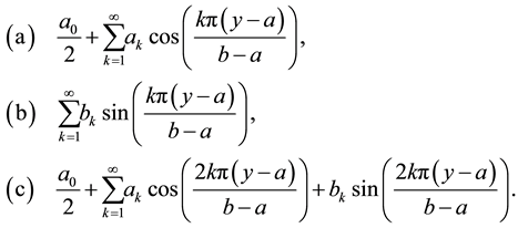 (1)
(1)
The use of the term “half-range” in describing Expressions (a) and (b) simply refers to the fact that the function![]() , although defined in
, although defined in![]() , has for the construction of the Fourier series been extended into the interval
, has for the construction of the Fourier series been extended into the interval
![]() as an even-valued function in the case of the half-range cosine series (so that sine contributions vanish) and as an odd-valued function in the case of the half-range sine series (so that the constant and cosine contributions vanish). Thus both half-range series are conventional Fourier series taken over the interval
as an even-valued function in the case of the half-range cosine series (so that sine contributions vanish) and as an odd-valued function in the case of the half-range sine series (so that the constant and cosine contributions vanish). Thus both half-range series are conventional Fourier series taken over the interval
![]() such that the function represented by the half-range Fourier cosine series is usually not differentiable at
such that the function represented by the half-range Fourier cosine series is usually not differentiable at![]() , whereas that represented by the half-range Fourier sine series is usually discontinuous at
, whereas that represented by the half-range Fourier sine series is usually discontinuous at![]() .
.
In the case of the half-range cosine and sine series in Expressions (1a) and (1b) respectively, the coefficients
![]() and
and
![]() are calculated from the function
are calculated from the function
![]() via the formulae
via the formulae
![]() (2)
(2)
in which

In terms of the exponential function the real coefficients
 and
and
 are calculated respectively as the real and imaginary parts of the single complex Equation
 (3)
(3)
In the case of the full-range Fourier series in Expression (1c) the real coefficients
 and
and
 are calculated respectively as the real and imaginary parts of the complex Equation
 (4)
(4)
Suppose now that
 is a transitional probability density function with known characteristic function defined formally by the Equation
 (5)
(5)
where
 and
and . A necessary condition for
 to be a probability density function is that
 as
as , and therefore there is guaranteed to be an interval
 such that for all
 it can be asserted that
 for any arbitrary small positive
 . The implication of this observation is that the Fourier coefficients in Equations (3) and (4) can be approximated from knowledge of the characteristic function via the respective formulae
 and
and , where
 (6)
(6)
while the coefficients of the full-range Fourier series can be approximated from knowledge of the characteristic function via the formula
 and
and , where
 (7)
(7)
The accuracy of approximations (6) and (7) is investigated in Section 6, where it is demonstrated that the error can be made arbitrarily small by choosing a suitably large interval.
3. Approximating Probability Density Functions
The quality of this practical idea is now explored for three trial probability density functions with known closed-form expressions for their characteristic functions. The first choice is the Gaussian density which may be regarded as representative of distributions with super-exponentially decaying tail density. The second and third choices are the Gamma density and the Cauchy density which are treated as representative examples of distributions with exponentially decaying and algebraically decaying tail densities respectively.
3.1. Gaussian Density
It is well known that the Gaussian density with mean value
 and variance
 has characteristic function
 . In order to demonstrate the quality with which the true probability density
 can be reconstructed from a truncated Fourier series of the form of Equation (1c), suppose that
 and take the interval of support to be
 , i.e. four standard deviations on either side of the mean value. The approximating function in this case using
 frequencies is
 (8)
(8)
where . Figure 1 illustrates the quality of this approximation using 40 frequencies (solid line,
 ) and using 4 frequencies (dashed line,
 ).
).
With as few as 4 frequencies it is clear that the approximating density still provides a good representation of the true density; with 40 frequencies the approximating density function is indistinguishable from the true density function, at least in terms of the resolution in Figure 1. It will be seen that this excellent performance is explained by the fact that the cumulative distribution function of the Gaussian probability density function converges to zero super-exponentially as
 and to unity as
 .
.
3.2. Gamma Density
The Gamma density with shape parameter
 and scale parameter
 has probability density function and characteristic function give by the respective formulae
 (9)
(9)
The approximating density is identical to Expression (8) with . The task is now to reconstruct the Gamma probability density function from
 . Because
 is also Gamma distributed, in this case with shape parameter
 and unit scale parameter, then the appropriate comparison for the Gamma distribution is between the approximating Fourier series and a Gamma distribution with unit scale parameter. Figure 2 illu-
strates the quality of this approximation for
 for 50 frequencies (solid line,
 ) and 20 frequen-
cies (dashed line, ). With the exception of the region very close to the origin, the true density and approximated density are not significantly different for even 20 frequencies, and with 50 frequencies the difference between the true density and the approximating density is not discernible with the exception of the origin which does not present a difficulty since the density to known to be zero there.
The quality of the approximation is again due to the fact that the cumulative distribution function of the Gamma density converges exponentially to zero as . Typical values for the coefficient of mean reversion (say,
 ), the mean volatility (say
 ) and the volatility of volatility (say
 ) in Heston’s model of stochastic volatility lead to a stationary distribution of volatility described by a Gamma density with shape parameter
 . A second example with
 and
and
 is illustrated in Figure 3.
The important observation from both of these experiments is that distributions with exponentially decaying tail density can also be well described by a relatively small range of frequencies.
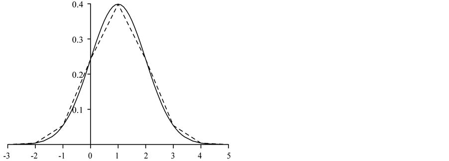
Figure 1. Comparison of the true Gaussian density and its approximation based on 40 frequencies (solid line, N = 80) and 4 frequencies (dashed line, N = 8).
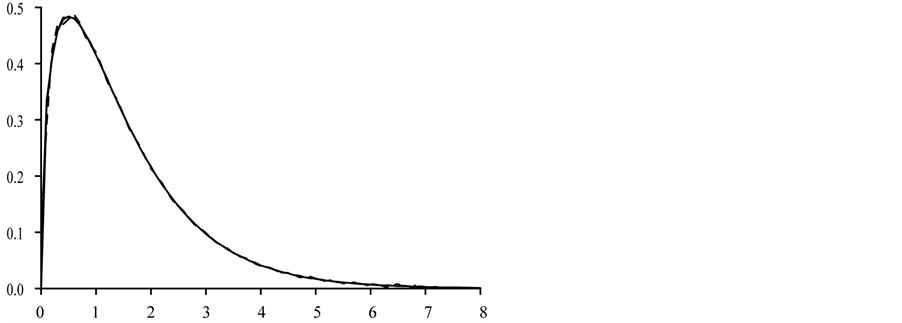
Figure 2. Comparison of the Gamma density
 and its approximations based on 50 frequencies (solid line, N = 100) and 20 frequencies (dashed line, N = 40).

Figure 3. Comparison of the Gamma density
 (solid line) and its approximations based on 10 frequencies (dashed line, N = 20).
3.3. Cauchy Density
The Cauchy density with median
 and scale parameter
 has probability density function and characteristic function give by the respective formulae
 (10)
(10)
The approximating density is again Expression (8) with . The task is now to reconstruct the Cauchy probability density function from
 , and for this purpose let
 ,
,
 and suppose that
 is treated as a function of compact support over the interval
 . The cumulative dis- tribution function of the Cauchy density is

which in this case converges algebraically to zero as
 and algebraically to unity as
 . Figure 4 illustrates the impact of this inferior rate of decay for the approximation based on 10 frequencies.
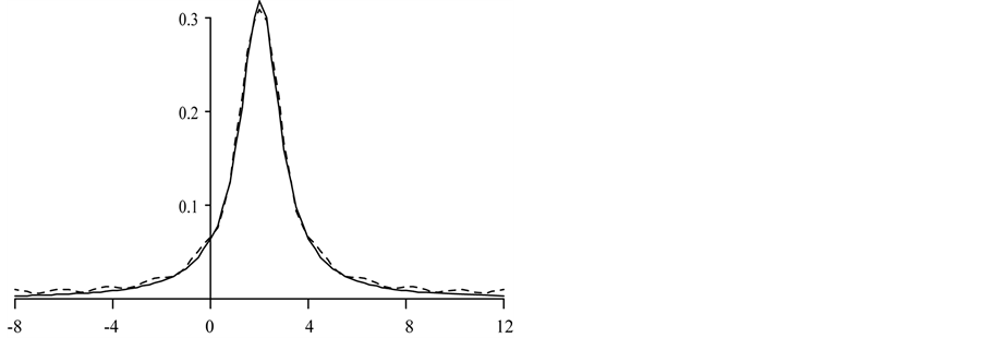
Figure 4. Comparison of the Cauchy density with parameters
 and
and
 (solid line) and the approximating Fourier series based on 10 frequencies (dashed line, N = 20).
While some erratic behaviour is evident in the tails of the approximating density, nevertheless the quality of the approximation is remarkably good considering the small number of frequencies in use.
In general, the approximate representations of the Gaussian, Gamma and Cauchy probability density functions all share the common fact that
 provides an upper bound for the error in the representation of density, where
 is the conventional cumulative distribution function of the underlying probability density function
 . In reality the error is significantly less than this upper bound due to cancellations resulting from the fact that the integrand in each of the Gaussian, Gamma and Cauchy densities is the product of a slowly varying probability density function decaying to zero and an independent rapidly oscillating function (in this case trigonometric functions represented in exponential form). However, the presence of this cancellation cannot change the character of the error which is entirely determined by the properties of
 as
as
 and as
 .
.
3.4. Comparison of True and Approximating Densities
While the illustrations of Figures 1-4 suggest that the Fourier series approximation of density is effective, it would be useful to quantify just how well density is approximated by the various Fourier methods. Instinctively it would seem that one possible way to achieve this objective is to use the Kullback-Leibler (KL) divergence criterion
![]() (11)
(11)
to measure the “distance” or departure of the probability density function
![]() from that of
from that of![]() , which in the formulation of Equation (11) is taken to be the true probability density function. The measure appeals to the fact that
, which in the formulation of Equation (11) is taken to be the true probability density function. The measure appeals to the fact that
![]() with equality if and only if the density functions
with equality if and only if the density functions
![]() and
and
![]() are identical. However, the KL criterion is simply an application of Jensen’s inequality for the concave function
are identical. However, the KL criterion is simply an application of Jensen’s inequality for the concave function![]() , and the properties of the criterion rely critically on the fact that
, and the properties of the criterion rely critically on the fact that
![]() and
and
![]() are probability densities, i.e. they are non-negative functions which integrate to unity.
are probability densities, i.e. they are non-negative functions which integrate to unity.
The central idea of each Fourier approximation is to replace the true probability density function by a function of compact support, that is,
![]() outside its interval of support. Consequently using measure (11) to compute the departure of the approximating density
outside its interval of support. Consequently using measure (11) to compute the departure of the approximating density
![]() from the true density
from the true density
![]() will typically require division by zero thereby rendering inappropriate the application of the KL criterion when used with
will typically require division by zero thereby rendering inappropriate the application of the KL criterion when used with
![]() as the true probability density. However, inverting the problem, one can use the KL criterion to measure the distance between the approximating density
as the true probability density. However, inverting the problem, one can use the KL criterion to measure the distance between the approximating density
![]() and the true density
and the true density![]() , that is, one may compute the value of
, that is, one may compute the value of
![]() in Expression (11) taking
in Expression (11) taking
![]() to be the approximating density and
to be the approximating density and
![]() to be the true density. In this case the integrand of expression (11) is well defined for all values of
to be the true density. In this case the integrand of expression (11) is well defined for all values of![]() , and therefore in order to proceed in this direction it remains to ensure that the approximating density integrates to unity. Approximations of density based on either the half range Fourier cosine series or the full range Fourier series are guaranteed to have this property, whereas an approximation based on the half range Fourier sine series need not share this property and therefore is inappropriate for analysis using the KL criterion. Tables 1-3 show values for the KL criterion for the Gaussian distribution with mean value one and unit standard deviation, the Gamma distribution with shape parameter 3 and scale parameter one, and the Cauchy distribution with median two and scale parameter one.
, and therefore in order to proceed in this direction it remains to ensure that the approximating density integrates to unity. Approximations of density based on either the half range Fourier cosine series or the full range Fourier series are guaranteed to have this property, whereas an approximation based on the half range Fourier sine series need not share this property and therefore is inappropriate for analysis using the KL criterion. Tables 1-3 show values for the KL criterion for the Gaussian distribution with mean value one and unit standard deviation, the Gamma distribution with shape parameter 3 and scale parameter one, and the Cauchy distribution with median two and scale parameter one.
As might be anticipated, the Gaussian distribution is most efficiently approximated by Fourier methods followed by the Gamma distribution and finally the Cauchy distribution. However, it is clear that all of these distributions are well approximated by the half range Fourier cosine and full range Fourier series for sufficiently large intervals of support and an adequate number of frequencies. The results in these tables also reinforce the

Table 1. Values of the KL measure (Dc for the half range Fourier cosine series and Df for the full Fourier series) are given for the Gaussian density with unit mean and unit standard deviation. Values measure the deviation of the true density deviates from the approximating density for intervals of length 6, 8, 10, 12 and 14 standard deviations centred about the mean of the Gaussian distribution using 5, 10, 25, 50, 100 and 200 frequencies.
Table 2. Values of the KL measure (Dc for the half range Fourier cosine series and Df for the full Fourier series) are given for the Gamma density with shape parameter 3 and unit scale factor. Values measure the deviation of the true density deviates from the approximating density for intervals [0, L] of length 6, 8, 10, 12 and 14 scale factors using 5, 10, 25, 50, 100 and 200 frequencies.
Table 3. Values of the KL measure (Dc for the half range Fourier cosine series and Df for the full Fourier series) are given for the Cauchy density with median two and unit scale factor. Values measure the deviation of the true density deviates from the approximating density for intervals of length 14, 20, 26, 32 and 38 scale factors centred about the median of the Cauchy distribution using 5, 10, 25, 50, 100 and 200 frequencies.
idea that the number of frequencies used in the approximation is of secondary importance to the size of the interval of support once sufficient frequencies are in use. This observation accords with intuition in the respect that larger intervals of support capture more of the true density and reduce the distortion in the approximating density, which as has already been commented, will always integrate to one. It would seem that approximations based on 50 frequencies are adequate in all of these examples. The results suggest that using more frequencies provides no meaningful improvement in accuracy. Moreover, for practical purposes there is little to choose between approximation based on the half range Fourier cosine and the full range Fourier series, although the latter has a slight edge for sufficiently large intervals and an adequate number of frequencies.
4. Pricing European Options
The successfully pricing of European option contracts for affine models of stochastic volatility requires knowledge of the marginal density of the asset price under the risk-neutral measure. The difficulty, however, is that no closed-form expression for this density is available for even the simplest of the multivariate affine models used in finance, although it is well known that such models have characteristic function,
![]() , of generic form
, of generic form
![]() (12)
(12)
where
![]() is the maturity of the option,
is the maturity of the option,
![]() is the backward variable and
is the backward variable and
![]() is the characteristic variable associated with the non-dimensional variable
is the characteristic variable associated with the non-dimensional variable![]() , here defined to be the logarithm of the ratio of asset price to strike price. The state variables
, here defined to be the logarithm of the ratio of asset price to strike price. The state variables
![]() in Expression (12) denote the values of the latent states of the system at time
in Expression (12) denote the values of the latent states of the system at time![]() . Typically the functions
. Typically the functions
![]() are the solution of a system of
are the solution of a system of
![]() ordinary differential Equations with initial conditions
ordinary differential Equations with initial conditions
![]() and
and![]() . In overview, there is a well trodden procedure that starts with the specification of the multivariate affine model and ends with the construction of
. In overview, there is a well trodden procedure that starts with the specification of the multivariate affine model and ends with the construction of![]() .
.
4.1. European Call Option
In the case of a European call option with strike price
![]() and maturity
and maturity
![]() on an asset with spot price
on an asset with spot price![]() , the price of the option is
, the price of the option is
![]()
where
![]() is the marginal density of the asset price at the maturity of the option when
is the marginal density of the asset price at the maturity of the option when
![]() is the spot price of the asset and
is the spot price of the asset and
![]() are the spot values of the latent states. When expressed in terms of
are the spot values of the latent states. When expressed in terms of![]() , the price of the option, say
, the price of the option, say![]() , becomes
, becomes
![]() (13)
(13)
where![]() . The value of this integral is now approximated under the assumption that
. The value of this integral is now approximated under the assumption that
![]() is well approximated by a function of compact support over the interval
is well approximated by a function of compact support over the interval![]() . Of course, the specific form taken by this approximation will depend of the choice of Expressions (a), (b) or (c) in Equations (1), but in each case the approximation of
. Of course, the specific form taken by this approximation will depend of the choice of Expressions (a), (b) or (c) in Equations (1), but in each case the approximation of
![]() by a function of compact support in
by a function of compact support in
![]() necessarily changes the interval of integration in Expression (13) from
necessarily changes the interval of integration in Expression (13) from
![]() to
to![]() . Thereafter it follows that the costs,
. Thereafter it follows that the costs,
![]() , of a call option on the basis of approximations (a) and (b) are respectively
, of a call option on the basis of approximations (a) and (b) are respectively
![]() (14)
(14)
where![]() . Based on approximation (c) the price of a call option is
. Based on approximation (c) the price of a call option is
![]() (15)
(15)
where![]() . The primary computational load in the computation of Expressions (a), (b) and (c) resides in the calculation of trigonometric functions, and consequently individual terms of Expression (c) require more arithmetical effort than the equivalent terms of either Expression (a) or (b). However the difference in computational load is minor when the more rapid convergence of summation (c) is compared with that of summations (a) and (b) simply because the frequencies used in approximation (c) are exactly double those used in approximations (a) and (b).
. The primary computational load in the computation of Expressions (a), (b) and (c) resides in the calculation of trigonometric functions, and consequently individual terms of Expression (c) require more arithmetical effort than the equivalent terms of either Expression (a) or (b). However the difference in computational load is minor when the more rapid convergence of summation (c) is compared with that of summations (a) and (b) simply because the frequencies used in approximation (c) are exactly double those used in approximations (a) and (b).
4.2. Binary Option
The price of a binary (call) option with strike price
![]() and maturity
and maturity
![]() on an asset with spot price
on an asset with spot price
![]() is
is
![]()
where
![]() is the marginal density of the asset price at the maturity of the option when the asset has spot price
is the marginal density of the asset price at the maturity of the option when the asset has spot price
![]() and
and
![]() are the spot values of the latent states. When expressed in terms of
are the spot values of the latent states. When expressed in terms of![]() , the price of the binary becomes
, the price of the binary becomes
![]() (16)
(16)
where![]() . The value of this integral is now approximated under the assumption that
. The value of this integral is now approximated under the assumption that
![]() is well represented by the procedures proposed in Section 2. Specifically, the price of a binary option computed from the half-range Fourier cosine and sine series are respectively
is well represented by the procedures proposed in Section 2. Specifically, the price of a binary option computed from the half-range Fourier cosine and sine series are respectively
![]() (17)
(17)
where![]() . The price of the binary option based on the full-range Fourier series (c) is
. The price of the binary option based on the full-range Fourier series (c) is
![]() (18)
(18)
where![]() . As is the case with the pricing of a call option, the frequencies used in approximation (c) are double those used in approximations (a) and (b) suggesting that calculations based on Expression (c) can be expected to converge more rapidly than those based on Expressions (a) and (b).
. As is the case with the pricing of a call option, the frequencies used in approximation (c) are double those used in approximations (a) and (b) suggesting that calculations based on Expression (c) can be expected to converge more rapidly than those based on Expressions (a) and (b).
5. The Heston Model of Stochastic Volatility
Heston’s [12] risk-neutral model of stochastic volatility has expression
![]() (19)
(19)
where![]() ,
,
![]() is the diffusion of asset price,
is the diffusion of asset price,
![]() is the risk-free rate of interest,
is the risk-free rate of interest,
![]() is the dividend rate,
is the dividend rate,
![]() is the risk-neutral rate of mean reversion of volatility to the risk-neutral long run value of
is the risk-neutral rate of mean reversion of volatility to the risk-neutral long run value of![]() ,
,
![]() scales the volatility of diffusion,
scales the volatility of diffusion,
![]() is the local correlation between returns and volatility and
is the local correlation between returns and volatility and
![]() are increments in the independent Brownian motions
are increments in the independent Brownian motions
![]() and
and![]() .
.
Suppose that
![]() is the probability density function of Equations (19) expressed in terms of the backward state
is the probability density function of Equations (19) expressed in terms of the backward state
![]() and the forward state
and the forward state![]() , then the backward Kolmogorov Equation satisfied by the transitional probability density function of Equations (19) is
, then the backward Kolmogorov Equation satisfied by the transitional probability density function of Equations (19) is
![]() (20)
(20)
Let
![]() be the characteristic function of
be the characteristic function of
![]() with respect to the forward variables, that is,
with respect to the forward variables, that is,
![]() (21)
(21)
By taking the Fourier transform of Equation (20) with respect to the backward variables, the characteristic function
![]() is seen to satisfy the partial differential Equation
is seen to satisfy the partial differential Equation
![]() (22)
(22)
with terminal condition
![]()
Thereafter, it is straightforward to show that the anzatz
![]() (23)
(23)
with
![]() is a solution of Equation (22) provided the coefficient functions
is a solution of Equation (22) provided the coefficient functions![]() ,
,
![]() and
and
![]() satisfy the ordinary differential equations
satisfy the ordinary differential equations
![]() (24)
(24)
The characteristic function of the marginal density of the terminal value of
![]() requires the solution of Equations (24) with initial conditions
requires the solution of Equations (24) with initial conditions![]() ,
,
![]() and
and
 for the particular values of
 needed to construct the half-range and full-range Fourier series approximations of transitional probability density.
On a practical note, the fact that the characteristic function of
 embeds the difference between the risk-free rate of interest and the dividend rate suggest at first sight that the coefficients
 must be computed whenever the risk-free rate or dividend rate changes, potentially each day, and not just when the parameters of the model are changed. The key to avoiding this difficulty is to note that the difference
 enters the calculation of
 alone, and that the behaviours of
 are independent of the behaviour of
 . Consequently, the resolution of this practical dilemma is to divide the calculation of
 into two stages with the first stage treating only those calculations that involve the difference
 and the second stage treating everything that is independent of the value of
 . Both stages are brought together each day in the calculation of the expected payoff, but only the first stage of calculation needs be done on a day-to-day basis. In particular, this calculation is very easy as it amounts to adding
 to the second stage calculation of
 in the computation of
 .
.
6. Error Analysis
Let
 denote the marginal density of
 , where
 denotes the strike price of an asset. The purpose of this section is to demonstrate that the error in estimating the price of a call option using only that part of the density
 in the finite interval
 can be made arbitrarily small by choosing a suitably large interval. The function
 , when truncated to the interval
 , is assumed to satisfy the Dirichlet conditions and therefore is guaranteed to have a convergent Fourier series on
 . The approximation procedure introduces three different errors which are now described.
6.1. Truncation Error
Truncation error occurs when the semi-infinite interval in Expression (13) or (16) is replaced by an integral over a finite interval, say
 in these expressions. With this approximation in place, the price of the call option is approximated by the expression
 (25)
(25)
resulting in an error due to the loss of the contribution to the price from values of
 in
in . A straightforward analysis indicates that the error in replacing the true cost of the call option by Expression (25) is

which in turn simplifies to give
 (26)
(26)
where
 is the cumulative function of
 . Evidently the truncation error in pricing a call option is the sum of two positive contributions, both of which are driven by the extent to which the restriction of the marginal density of
 to the interval
 fails to capture density in the upper tail of the distribution of Y. Thus Expression (25) with a numerically accurate representation of the true marginal density of
 will always underestimate the true value of a call option, although the error can be made arbitrarily small by taking
 to be a suitably large interval.
The inference from this observation is that approximations of
 which place unit density in
 may potentially compensate for some of the error incurred in using the truncation procedure to price a call option. The half-range Fourier cosine and full-range Fourier series approximations of transitional probability density both fall into this category, which in turn suggests that the use of the truncation procedure with these approximations of marginal density may well provide rather smaller pricing errors than might casually be anticipated. By contrast, the half-range Fourier sine series approximation of marginal density does not capture unit density in the interval
 , and the corresponding conjecture is that this approximation of marginal density will perform less well than the half-range Fourier cosine and full-range Fourier series approximations with regard to the pricing of a call option. Table 4 indicates that this conjecture is borne out in practice.
6.2. Approximation Errors
Suppose now that the transitional density
 in the interval
 is replaced by the Fourier series
 (27)
(27)
where the choice of frequencies
 and the values of
 ,
,
 depend on the choice of Fourier representation. Two errors arise in the calculation of Expression (25). First, the plan is to replace the coefficients
 in Equation (27) by the misspecified coefficients
 computed directly from the characteristic function
 of
of
 via the formula
(a)
(b)
(c)
Table 4. Percentage errors recorded by the half-range cosine series, half-range sine series and full-range Fourier series of pricing a European call option and a binary option with strike K = 1200 and maturities one month (panel (a)), three months (panel (b)) and six months (panel (c)). The factor refers to the multiple of
 used to establish the interval over which to compute the numerical approximation.
 (28)
(28)
Consequently a misspecification error arises in the Fourier coefficients. Second, the truncation of the Fourier series (27) to a finite number of terms, say
 terms, introduces another approximation error. Therefore the price of a call option based on this strategy is
 (29)
(29)
in which
 in Expression (25) has been replaced by the first
 terms of the Fourier series (27) with misspecified coefficients
 and
and . The error introduced by this approximation is
 (30)
(30)
which has explicit expression
 (31)
(31)
The misspecification error in the coefficients
 and
and
 due to the use of the coefficients
 and
and
 respectively is determined from the identity

Standard properties of integral Calculus guarantee that

where
 (32)
(32)
It therefore follows directly that
 (33)
(33)
for all values of . Thus the misspecification error in the Fourier coefficients is driven entirely by the choice of interval
 via the magnitude of the cumulative function
 at
at
 and
and . In practice this error will be significantly smaller than the maximum bound given in Equation (33) as a result of arithmetical cancellation due to the oscillatory nature of the integrand, but as commented previously, the decay of this error as
 will be determined by the behaviour of
 as
as
 and as
 .
.
In conclusion, the total error in pricing a call option, namely
 (34)
(34)
is formed by connecting together Equation (26) for the error arising in the truncation of the density
 to the finite interval
 , Equation (29) for the value of the option in terms of the misspecified Fourier coefficients
 , and Equation (31) for the size of the resulting misspecification error in the option price. The result is that the error is
 (35)
(35)
Each integral is replaced by its value and the triangle inequality is used to deduce that
 (36)
(36)
The contributions to the error from the first, second, third and fourth terms on the right hand side of inequality (36) are dominated by the behaviour of
 and
and . By choosing the interval
 suitably large,
 and
and
 can be made arbitrarily small. The behaviour of the fifth and sixth terms on the right hand side of inequality (36) depends on the choice of
 . Bearing in mind that
 , then it straightforward to show that there are positive constants
 and
and
 such that
The well known result that if
 is a continuous function3 of
 , then
 and
and
 indicates that the fourth and fifth terms of inequality (36) are
 and
and
 respectively. Thus the fifth and sixth terms on the right hand side of inequality (36) can also be made arbitrarily small by a suitably large choice of
 .
.
In conclusion, the error in pricing a call option can be made arbitrarily small by restricting the marginal probability density to a finite interval
 and approximating the density in that interval by a misspecified Fourier series constructed from the characteristic function at the appropriate frequencies.
7. Performance under Simulation
A series of simulation experiments was undertaken in order to examine the efficacy of the half-range Fourier cosine series, half-range Fourier sine series and full-range Fourier series in respect of how accurately these approximations price European call options and binary options. The first experiment prices options in a Black- Scholes world so that a closed-form solution may be used to assess the pricing error, whereas the second experiment prices the same options using Heston’s model of stochastic volatility.
7.1. Black-Scholes Pricing
Assume that the asset price,
 , follows a geometric Brownian motion

in which
 is the increment of a Wiener process. The advantage of using this specification is that, following the seminal work of Black and Scholes [13] , exact prices are known for each type of option for all combinations of spot price
 , strike price
 , and maturity
 . It follows, therefore, that the relative percentage pricing error incurred using numerical methods based on Fourier series for a variety of different strike prices and maturities can be identified exactly.
Three major experiments are performed. In each of these experiments ,
,
 per year,
 and the strikes
 are taken to be 1200, 1000 and 800 respectively so as to examine the performance of the algorithms when the options are out-of-the-money, at-the-money and in-the-money. In each simulation the accuracy of the various approximations of transitional density is assessed for prescribed values of
 and
and
 in which the size of the interval
 is expressed as a multiple of
 ranging from 5 to 9. The results of these exercises are reported in Tables 4-6 with each table reporting the results for maturities of one month (panel (a)), three months (panel (b)) and six months (panel (c)).
Two very clear general conclusions emerge from these results.
1) For options that are deep in-the-money (Table 6) in which
 and
and , or at-the-money (Table 5) in which
 and K = 1000, it matters little (if at all) which of these three pricing algorithms are chosen irrespective of the maturity of the option. Indeed the relative pricing error is zero for all practical purposes.
2) For options that are deep out-of-the-money (Table 4) in which
 and
and , the choice of algorithm is more important. The results may be summarized succinctly as follows.
a) The half-range Fourier sine series does not perform as well as the other two approximations and its use is therefore not recommended. This finding accords well with our previous intuition based on a consideration of the contribution to the price of a call option lost as a result of truncating marginal density.
b) The half-range Fourier cosine series and the full-range Fourier series both perform relatively well. When the size of the interval of approximation is a relatively small multiple of , namely either 5 or 6, then the half-range Fourier cosine series performs better that the full-range Fourier series. As the multiple of
 increases and the size of the interval of approximation becomes larger, the full-range Fourier series begins to dominate. When the interval of approximation has size
 , then the full-range Fourier series is unambiguously superior to the half-range Fourier cosine series, particularly for options of short maturity.
On the basis of this analysis and on accuracy grounds, it is hard to ignore the claim that the full-range Fourier series is the algorithm of choice when using Fourier methods to price options. Moreover, the full-range Fourier series converges faster than either the half-range sine or cosine series and is therefore likely to price options more rapidly. These themes are explored in more detail in the pricing of call options under Heston’s model of stochastic volatility.
7.2. Heston’s Model
A total of approximately 40,000 options over ten years were generated by simulation of Heston’s model. Sixteen
(a)
(b)
(c)
Table 5. Percentage errors recorded by the half-range cosine series, half-range sine series and full-range Fourier series of pricing a European call option and a binary option with strike K = 1000 and maturities one month (panel (a)), three months (panel (b)) and six months (panel (c)). The factor refers to the multiple of
 used to establish the interval over which to compute the numerical approximation.
options were generated each day spread over 4 maturities ranging from 92 to 5 days and 4 strikes two of which are initialised at 20% out of and into the money and two of which are initialised at 7% out of and into the money. The half-range Fourier cosine series and the full-range Fourier series are then used to price call options and binary options with these strikes. In this instance no exact solutions are available, and so the accuracy of each method in respect of each type of option is gauged by comparison against values calculated using a large interval. The left hand and middle columns of Table 7 show respectively the
 and
and
 relative pricing errors for out-of-the-money call options calculated using the half-range Fourier cosine series and the full-range Fourier series. The right hand column of Table 7 shows the CPU time (secs) needed to perform the calculations. The left hand column specifies the length of the interval
 in multiples of
 , the unconditional standard deviation of the distribution of
 about
about
 after an interval of duration
 , taken to be a trading day in the simulation study, i.e.
 .
.
A clear finding from Table 7 is that the half-range Fourier cosine series performs well in respect of the
 measure for shorter intervals and in the
 measure for almost all choices of interval length. By contrast the
(a)
(b)
(c)
Table 6. Percentage errors recorded by the half-range cosine series, half-range sine series and full-range Fourier series of pricing a European call option and a binary option with strike K = 800 and maturities one month (panel (a)), three months (panel (b)) and six months (panel (c)). The factor refers to the multiple of
 used to establish the interval over which the numerical approximation is computed.
performance of the full-range Fourier series is poor with regard to both measures for shorter intervals. However, the quality of approximation provided by the half-range cosine series is erratic as the size of the Fourier window increases whereas that provided by the full-range Fourier series improves systematically to the extent that its performance surpasses that of the half-range Fourier cosine series for intervals of length 24 standard deviations or more. Furthermore, this level of accuracy is achieved by the full-range Fourier series in approximately 25% quicker than that required by the half-range Fourier cosine series.
Fang and Oosterlee [10] suggest choosing intervals of length 20 standard deviations. In this problem, it is evident that the half-range Fourier cosine series still enjoys an advantage over the full-range Fourier series for intervals of this length. The suggestion of this investigation is that 20 standard deviations should be regarded as a minimum length of interval. Table 8 shows the
 and
and
 relative pricing errors calculated from the half- range Fourier cosine series and the full-range Fourier series in respect of in-the-money call options based on Heston’s model.
Table 7. The L2 and L1 relative pricing errors calculated from the half-range Fourier cosine series and the full-range Fourier series for out-of-the-money call options based on Heston’s model. The timings refer to the times (seconds) needed to price 12 daily call options over 10 years with maturities ranging from 5 to 92 days. The factor refers to the multiple of σY used to establish the interval over which the numerical approximation is computed.
Table 8. The L2 and L1 relative pricing errors calculated from the half-range cosine series and the full-range Fourier series for in-the-money call options based on Heston’s model. The timings refer to the times (seconds) needed to price 12 daily call options over 10 years with maturities ranging from 5 to 92 days. The factor refers to the multiple of σY used to establish the interval over which the numerical approximation is computed.
The results reported in Table 8 exhibit a similar pattern of behaviour to those reported in Table 7, namely that for intervals of short length the half-range Fourier cosine series outperforms the full-range Fourier series with respect to both the
 and
and
 measures of accuracy, but that this dominance vanishes when the length of the interval of approximation is 24 standard deviations or more. In particular, both approaches generate noticeably smaller relative errors for in-the-money options than for out-of-the-money options. Because in-the-money call options carry a higher price, one inference of this observed reduction in relative error is that the absolute pricing error in using each Fourier representation is insensitive to the moneyness of the option. Table 8 and Table 9 report the performance of the half-range Fourier cosine series and the full-range Fourier series when used to price binary options.
The results presented in Table 9 and Table 10 demonstrate that both the half-range Fourier cosine series and the full-range Fourier series both generate good estimates of the price of binary options with the former performing better than the latter for intervals of short length, but with this advantage disappearing when the length of the interval is increased.
Table 9. The L2 and L1 relative pricing errors calculated from the half-range cosine series and the full-range Fourier series for out-of-the-money binary options based on Heston’s model. The timings refer to the times (seconds) needed to price 12 daily call options over 10 years with maturities ranging from 5 to 92 days. The factor refers to the multiple of σY used to establish the interval over which the numerical approximation is computed.
Table 10. The L2 and L1 relative pricing errors calculated from the half-range cosine series and the full-range Fourier series for in-the-money binary options based on Heston’s model. The timings refer to the times (seconds) needed to price 12 daily call options over 10 years with maturities ranging from 5 to 92 days. The factor refers to the multiple of σY used to establish the interval over which the numerical approximation is computed.
The results reported in Tables 7-10 are characterised by two common denominators. First, the computational time required by the half-range Fourier cosine series is uniformly longer than that required by the full-range Fourier series for an interval of fixed length. The simple explanation for this observation is that the full-range Fourier series uses larger frequencies for a given length of interval, and therefore the full-range Fourier series converges more rapidly. Second, the pricing of call options and binary options using the half-range Fourier cosine series representation of transitional density is noticeably better than the corresponding pricing using the full-range Fourier series for short intervals , but this advantage vanishes in the case of the binary option when the interval becomes suitably large and is reversed in the case of a call option. The primary explanation for this behaviour lies in the realisation that tail density is characterised by long wavelengths, or equivalently by the presence of low frequency terms, whereas peaky density is characterised by short wavelengths, or equivalently high frequency terms.
For an interval of given length, the frequencies present in the half-range Fourier cosine expansion are smaller that the frequencies present in the full-range Fourier series, and therefore when the length of the interval
 is small, the half-range Fourier cosine series better captures tail behaviour. Increasing the length of the interval lowers the range of frequencies admitted to the full-range Fourier series expansion, which in turn improves its ability to handle tail density. However, the same increase in length will benefit the half-range Fourier cosine series representation of transitional density only provided there remains significant tail density to be characterised by these new frequencies. On the other hand, the half-range Fourier cosine series will always suffer from the drawback that the (periodic) function it represents has gradient zero at
 and
and
 (because the series is not generally differentiable at these points). Consequently, the half-range Fourier cosine series approximation will always misrepresent the gradient of the true density function at
 and
and
 in contrast to the behaviour of the approximation provided by the full-range Fourier series.
8. Conclusion
One clear conclusion from these calculations is that the half-range Fourier cosine series and the full-range Fourier series perform uniformly better than the half-range Fourier sine series. The half-range Fourier cosine series and the full-range Fourier series both perform with credit. When the length of the interval
 is relatively small, say ten or so standard deviations, it is clear that the half-range Fourier cosine series outperforms the full-range Fourier series over the same interval. On the other hand for intervals of larger length the full-range Fourier series is at least as good as the half-range Fourier cosine series, and outperforms the latter in pricing out-of-the-money call options, in particular, with maturities of three months or less. In general the full-range Fourier series outperforms the half-range Fourier cosine series in all circumstances provided that the interval
 is suitably large, although the effect is so small as not to be significant in practice. The explanation for this behaviour lies in the fact that the half-range Fourier cosine series, although not representing a differentiable function, always uses a lower spectrum of frequencies than the full-range Fourier series and therefore enjoys an initial advantage in describing tail density. As the interval length is increased, this advantage vanishes. On the other hand the larger spectrum of the full-range Fourier series guarantees more rapid convergence. Of course, timing issues may not be important if small numbers of model call prices are to be calculated, but when facing calibration problems or estimation problems as described in the introductory remarks, timing issues are indeed significant once adequate numerical accuracy is assured.
References
- Johannes, M.S., Polson, N.G. and Stroud, J.R. (2009) Optimal Filtering of Jump Diffusions: Extracting Latent States from Asset Prices. Review of Financial Studies, 22, 2759-2799. http://dx.doi.org/10.1093/rfs/hhn110
- Broadie, M., Chernov, M. and Johannes, M. (2007) Model Specification and Risk Premia: Evidence from Futures Options. Journal of Finance, 62, 1453-1490. http://dx.doi.org/10.1111/j.1540-6261.2007.01241.x
- Christoffersen, P., Jacobs, K. and Mimouni, K. (2010) Volatility Dynamics for the S&P500: Evidence from Realized Volatility, Daily Returns and Option Prices. Review of Financial Studies, 23, 3141-3189. http://dx.doi.org/10.1093/rfs/hhq032
- Hurn, A.S., Lindsay, K.A. and McClelland, A.J. (2012) Estimating the Parameters of Stochastic Volatility Models Using Option Price Data. Unpublished Working Paper, NCER.
- Andersen, T.G., Fusari, N. and Todorov, V. (2012) Parametric Inference and Dynamic State Recovery from Option Pa- nels. NBER Working Paper Series.
- Carr, P.P. and Madan, D.B. (1999) Option Evaluation Using the Fast Fourier Transform. Journal of Computational Fi- nance, 2, 61-73.
- Borak, S., Detlefsen, K. and Hardle, W. (2005) FFT Based Option Pricing. SFB Discussion Paper 649.
- Lord, R., Fang, F. Bervoets, F. and Oosterlee, C.W. (2007) A Fast and Accurate FFT-Based Methodology for Pricing Early-Exercise Options under Levy Processes. SIAM Journal of Scientific Computing, 20, 1678-1705.
- Kwok, Y.K., Leung, K.S. and Wong, H.Y. (2012) Efficient Options Pricing Using the Fast Fourier Transform. In: Duan, J.C., Ed., Handbook of Computational Finance, Springer, Berlin, 579-604. http://dx.doi.org/10.1007/978-3-642-17254-0_21
- Fang, F. and Oosterlee, C.W. (2008) A Novel Pricing Method for European Options Based on Fourier-Cosine Series Expansions. SIAM Journal on Scientific Computing, 31, 826-848. http://dx.doi.org/10.1137/080718061
- Zhang, B., Grzelak, L.A. and Oosterlee, C.W. (2012) Efficient Pricing of Commodity Options with Earlyexercise under the Ornstein-Uhlenbeck Process. Applied Numerical Mathematics, 62, 91-111. http://dx.doi.org/10.1016/j.apnum.2011.10.005
- Heston, S.L. (1993) A Closed-Form Solution for Options with Stochastic Volatility with Applications to Bond and Cu- rrency Options. Review of Financial Studies, 6, 327-343.
- Black, F. and Scholes, M. (1973) The Pricing of Options and Corporate Liabilities. Journal of Political Economy, 81, 637-654. http://dx.doi.org/10.1086/260062
NOTES

1The Finite Fourier Transform is the integral expression defining the coefficients of a Fourier series.
2Historically, half-range Fourier series have largely arisen as analytical tools for handling various types of boundary conditions when solving partial differential equations using integral transforms.

3Sharper results can be obtained if
 for
for . However the function represented by the half-range Fourier cosine series is not generally differentiable at
 , and so the convergence argument is based on the weakest condition satisfied by Fourier coefficients.