Abstract

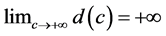
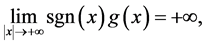
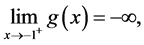
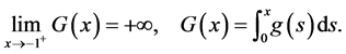
This paper is devoted to the study of second-order Duffing equation with singularity at the origin, where tends to positive infinity as, and the primitive function as. By applying the phase-plane analysis methods and Poincaré-Bohl theorem, we obtain the existence of harmonic solutions of the given equation under a kind of nonresonance condition for the time map.

Keywords:Harmonic Solutions, Duffing Equation, Singularity, Time Map, Poincaré-Bohl Theorem

1. Introduction

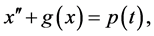
We deal with the second-order Duffing equation

(1)

where is locally Lipschitzian and has singularity at the origin, is continuous and periodic. Our purpose is to establish existence result for harmonic solution of Equation (1). Arising from physical applications (see [1] for a discussion of the Brillouin electron beam focusing problem), the periodic solution for equations with singularity has been widely investigated, referring the readers to [2] -[6] and their extensive references.

As is well known, time map is the right tool to build an approach to the study of periodic solution of Equation (1) (see [7] -[9] ). However, the work mainly focused on the equations without singularity. Our goal in this paper is to study the periodic solution of Equation (1) with singularity via time map. There is a little difference between our time map and the time map in [7] [9] . We now introduce the time map.

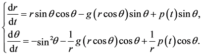
Consider the auxiliary autonomous system

(2)

and suppose that

Obviously, the orbits of system (2) are curves determined by the equation

where is an arbitrary constant.

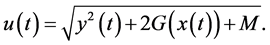
In view of the assumptions (g₀), (g₁) and (G₀), there exists a, such that for, is a closed curve. Let be a solution of (2) whose orbit is. Then this solution is periodic, denoting by the least positive period of this solution. It is easy to see that

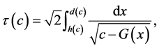(3)

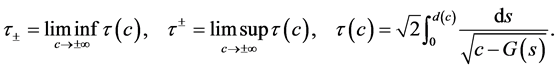
where, , ,.

We recall an interesting result in [7] . Ding and Zanolin [7] proved that Equation (1) without singularity possesses at least one T-periodic solution provided that

and a kind of nonresonance condition for the time map

(4)

where

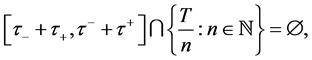
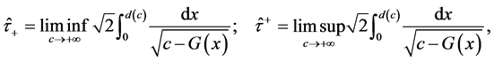
Now naturally, we consider the question whether Equation (1) has harmonic solution when we permit

cross resonance points and use a kind of nonresonance condition for time map. In the following we will give a positive answer. In order to state the main result of this paper, set

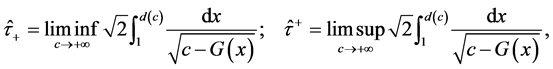(5)

and assume that

Our main result is following.

Theorem 1.1 Assume that, and hold, then Equation (1) has at least one 2π- periodic solution.

In this case, we generalize the result in [7] to Equations (1) with singularity.

The remainer of the paper is organized as follows. In Section 2, we introduce some technical tools and present all the auxiliary results. In Section 3, we will give the proof of Theorem 1.1 by applying the phase-plane analysis methods and Poincaré-Bohl fixed point theorem.

2. Some Lemmas

we assume throughout the paper that is locally Lipschitz continuous. In order to apply the phase-plane analysis methods conveniently, we study the equation

(6)

where is continuous and has a singularity at. In fact, we can take a parallel translation to achieve the aim. Then the conditions and become

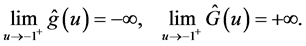
Dropping the hats for simplification of notations, we assume that

and

Thus,

(7)

and and in (3) satisfy

We will prove Theorem 1.1 under conditions, and instead of conditions, and.

Consider the equivalent system of (6):

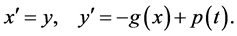(8)

Let be the solution of (8) satisfying the initial condition

We now follow a method which was used by [4] [6] and shall need the following result.

Lemma 2.1 Assume that conditions and hold. They every solution of system (8) exists uniquely on the whole t-axis.

By Lemma 2.1, we can define Poincaré map as follows

It is obvious that the fixed points of the Poincaré map correspond to -periodic solutions of system (8). We will try to find a fixed point of. To this end, we introduce a function,

Lemma 2.2 Assume that and hold. Then, for any, there exists sufficiently large that, for,

where is the solution of system (8) through the initial point.

This result has been proved in [6] and we omit it.

Using Lemma 2.2, we see that for if is large enough. Therefore, transforming to polar coordinates, , system (8) becomes

(9)

Denote by the solution of (9) with

Thus, we can rewrite the Poincaré map in the form

where.

For the convenience, two lemmas in [6] will be written and the proof can be found in [6] .

Lemma 2.3 Assume that and hold. Then there exists a such that, for,.

Lemma 2.4 Assume that, and hold. Then there exists a such that, for,

is a star-shaped closed curve about the origin.

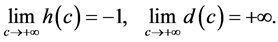
Lemma 2.5 Assume that, and hold. Denote by the time for the solution to make one turn around the origin. Then as, where and are given in (7).

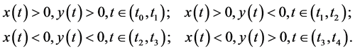
Proof. Without loss of generality, we may assume that. From Lemma 2.3, we have for sufficiently large and. Hence, there exist such that

, and

Throughout the lemma, we always assume that is large enough.

(1) We shall first estimate and. We can refer to Lemma 2.6 in [6] and obtain, as.

(2) We now estimate and. According to conditions and, we can choose a constant such that for. Set

(10)

Then,

Therefore, for,

Note that, we get

Since, we have

where. By condition, we know that increases for x sufficiently large, and tends to as. Therefore, there exist constants such that

(11)

By (10) and (11), we have

(12)

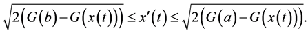
Let be such that, and. Following (12), we derive

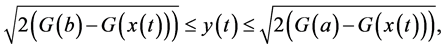(13)

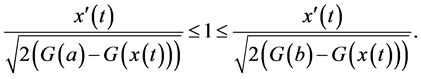
that is,

Consequently,

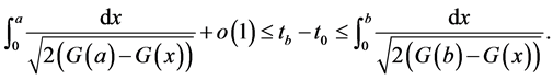
Integrating both sides of the above inequality from to, we obtain

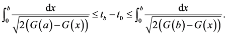(14)

Recalling the conditions and (11), we know that there is, such that. Applying Lemma 2.8 in [6] , we can derive

(15)

for. Combining (14) and (15), we have

From [10] , we know that

for. Hence,

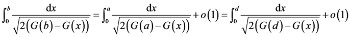
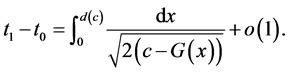
In the following, we deal with. Integrating 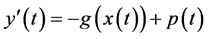from to, we get

(16)

By (13), we derive

(17)

On the other hand, from (11) we have

As a result,

Accordingly,

(18)

Meanwhile, following, for any given sufficiently large, there exist large enough, such that

(19)

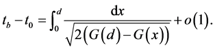
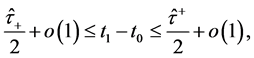
Combining (16)-(19), we get

for, where. Thus,

(20)

Using the same arguments as above, we can get

(21)

By the conditions (20), (21), we have

Recalling, , we have

The proof is complete.

3. Proof of Theorem 1.1

In this section, we establish the existence of harmonic solutions for Equation (1) by appealing to Poincaré-Bohl theorem [11] . We consider the Poincaré map

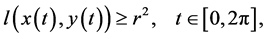
From Lemma 2.5 and condition, we obtain

which implies

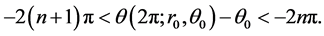
Thus, the image cannot lie on the line. Therefore, the Poincaré-Bohl theorem guarantees that the map has at least one fixed point, i.e. Equation (6) has at least one -periodic solution.

References

- Ding, T. (2004) Applications of Qualitative Methods of Ordinary Differential Equations. Higher Education Press, Beijing.
- Fonda, A. (1993) Periodic Solutions of Scalar Second-Order Differential Equations with a Singularity . Académie Royale de Belgique. Classe des Sciences. Mémoires, 8-IV, 68-98.
- Lazer, A.C. and Solimini, S. (1987) On Periodic Solutions of Nonlinear Differential Equations with Singularities. Proceedings of the American Mathematical Society, 99, 109-114. http://dx.doi.org/10.1090/S0002-9939-1987-0866438-7
- Wang, Z. (2004) Periodic Solutions of the Second Order Differential Equations with Singularity . Nonlinear Analysis: Theory, Methods & Applications, 58, 319-331. http://dx.doi.org/10.1016/j.na.2004.05.006
- Wang, Z., Xia, J. and Zheng, D. (2006) Periodic Solutions of Duffing Equations with Semi-Quadratic Potential and Singularity. Journal of Mathematical Analysis and Applications, 321, 273-285. http://dx.doi.org/10.1016/j.jmaa.2005.08.033
- Xia J. and Wang, Z. (2007) Existence and Multiplicity of Periodic Solutions for the Duffing Equation with Singularity. Proceedings of the Royal Society of Edinburgh: Section A Mathematics, 137, 625-645.
- Ding T. and Zanolin, F. (1991) Time-Maps for the Solvability of Periodically Perturbed Nonlinear Duffing Equations. Nonlinear Analysis: Theory, Methods & Applications, 17, 635-653. http://dx.doi.org/10.1016/0362-546X(91)90111-D
- Ding, T. and Zanolin, F. (1993) Subharmonic Solutions of Second Order Nonlinear Equations: A Time-Map Approach. Nonlinear Analysis: Theory, Methods & Applications, 20, 509-532. http://dx.doi.org/10.1016/0362-546X(93)90036-R
- Qian, D. (1993) Times-Maps and Duffing Equations Crossing Resonance Points . Science in China Series A: Mathematics, 23, 471-479.
- Capietto, A. Mawhin, J. and Zanolin, F. (1995) A Continuation Theorem for Periodic Boundary Value Problems with Oscillatory Nonlinearities. Nonlinear Differential Equations and Applications, 2, 133-163. http://dx.doi.org/10.1007/BF01295308
- Lloyd, N.G. (1978) Degree Theory. University Press, Cambridge.