Applied Mathematics
Vol.3 No.12(2012), Article ID:25589,5 pages DOI:10.4236/am.2012.312266
Generalized Minimum Perpendicular Distance Square Method of Estimation
Department of Statistics, Jahangirnagar University, Savar, Bangladesh
Email: rezaul@juniv.edu, Morshed@juniv.edu, munirhc@yahoo.com, forhad.ju88@yahoo.com
Received September 22, 2012; revised October 22, 2012; accepted October 30, 2012
Keywords: Heteroscedasticity; Ordinary Least Square Method; Minimum Perpendicular Distance Square Method; Generalized Least Square Method
ABSTRACT
In case of heteroscedasticity, a Generalized Minimum Perpendicular Distance Square (GMPDS) method has been suggested instead of traditionally used Generalized Least Square (GLS) method to fit a regression line, with an aim to get a better fitted regression line, so that the estimated line will be closest one to the observed points. Mathematical form of the estimator for the parameters has been presented. A logical argument behind the relationship between the slopes of the lines  and
and  has been placed.
1. Introduction
Linear regression has a long history in its way of development from the very begging of eighteenth century till today. A lot of literatures are available in this area, these literatures involves the estimation of regression coefficients and constant by Ordinary Least Square (OLS) method i.e. by minimizing the sum of square of the vertical distances between the observed points and the assumed regression line, and estimate the regression coefficients traditionally known as OLS estimation procedure.
M. F. Hossain and G. Khalaf, (2009) showed that OLS method does not minimize actual distance from the observed point to the fitted regression line. They have suggested minimum perpendicular distance square (MPDS) Method estimation for simple linear regression in case of homoscedasticity which boils down the traditional OLS method. But regression disturbances whose variances are not constant across observations are heteroscedastic. Heteroscedasticity arises in numerous applications, in both cross-section and time-series data. For example, even after accounting for firm sizes, we expect to observe greater variation in the profits of large firms than in those of small ones. The variance of profits might also depend on product diversification, research and development expenditure, and industry characteristics and therefore might also vary across firms of similar sizes. When analyzing family spending patterns, we observe greater variation in expenditure on certain commodity groups among high-income families than low ones due to the greater discretion allowed by higher incomes [1]. MPDS method is not suitable for this type of heteroscedasticity situation because this method was established only for homoscedasticity cases.
In this paper we have considered minimum perpendicular distance square method in case of heteroscedasticity which we called Generalized Minimum Perpendicular Distance Square (GMPDS) method.
2. Problems of Ordinary Least Square (OLS) and Generalized Least Square (GLS) Method
Suppose the simple linear regression model is
where the response variable ![]() is related to the explanatory variable
is related to the explanatory variable  through the regression coefficient
 , constant intercept
  and random disturbance term
![]() . We assume that the disturbance terms
. We assume that the disturbance terms  follow all assumptions of classical linear regression model.
The estimation procedure of regression coefficient by Ordinary Least Square (OLS) method and Generalized Least Square (GLS) method is actually minimizing the sum of square of the vertical distances  from the observed points to the assumed regression line.
The OLS estimators are:

and 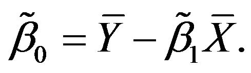
The important assumption for applying OLS method is that the variance of each disturbance term , conditional on the chosen values of the explanatory variables, is some constant number (is called homoscedasticity assumption). If the data violet this homoscedasticity assumption that is the variance of each disturbance term
  conditional on the chosen values of the explanatory variables is random (say
 ) then we can not apply OLS and in this case we apply GLS estimation procedure for estimating parameters [2].
The GLS estimators are:
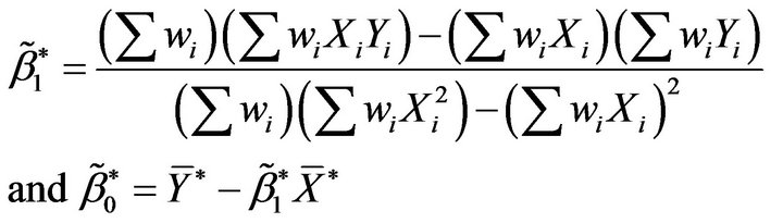
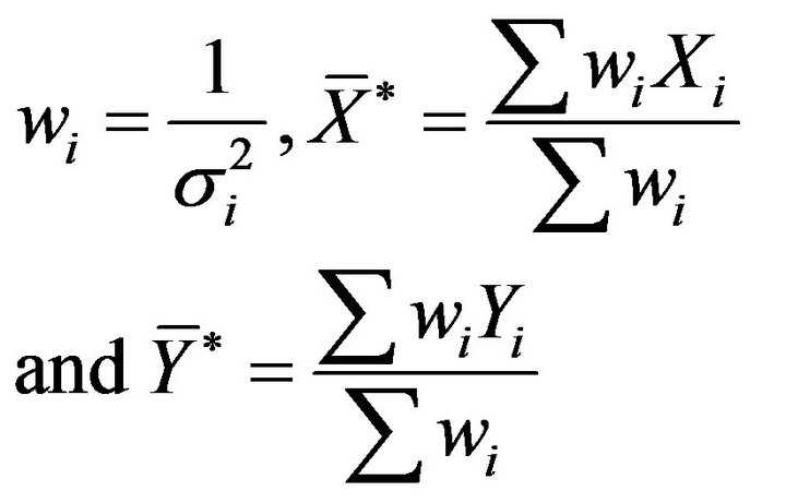
where,
The problem of OLS and GLS estimation is that, actually they don’t minimize real distance from the observed point to the fitted regression line rather they minimize the vertical distance from the observe point to the fitted regression line. For this reason we have the well known theorem is
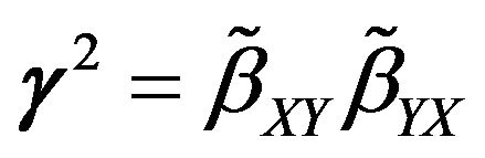 .
.
where  is the estimated regression coefficient of
  on
on ![]() and
and  is the estimated regression coefficient of
 ![]() on
on . If OLS and GLS minimize real distance (error) then
  should be unity that is
 . But in OLS and GLS methods, it only occurs if data are perfectly correlated, that is
 . In real life problem this type of perfect correlation occurs in rare case.
The Minimum Perpendicular Distance Square Method suggested by Hossain and Khalaf (2009) produced the estimator which gives  for all cases and it indicates that the errors are really minimized and gives more accurate result than that of OLS [3].
Concept of Minimum Perpendicular Distance Square (MPDS) Estimation
The real distance of the assumed regression line  from the points
  are not the vertical distances or height of the point minus height of regression line i.e.
 .
.
In fact the actual distances from the line  to the points
  are the perpendicular distances
 ’s (as indicated in Figure 1). These perpendicular distances would also be positive and negative according to
  is above the line
  or below the line
 . Also assuming that
 . Hence estimating
  and
and  by minimizing sum of the squares of these perpendicular distances will produce the closest fitted regression line from the points
  which may be used for more accurate prediction purposes.
3. The Method of Generalized Minimum Perpendicular Distance Squares Method (GMPDSM)
Let us consider two-variable linear regression function is

which for ease of algebraic simplification we write as
 (1)
(1)
where  for each
  and the response variable
 ![]() is related to the explanatory variable
is related to the explanatory variable  through the regression coefficient
 , constant intercept
  and random disturbance term
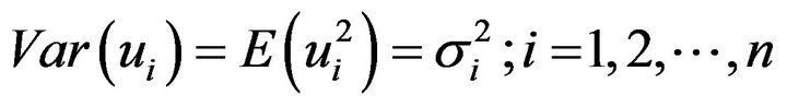
![]() . We know that one of the important assumptions of the classical linear regression model is that the variance of each disturbance term
. We know that one of the important assumptions of the classical linear regression model is that the variance of each disturbance term , conditional on the chosen values of the explanatory variables is some constant number equal to
 . This is the assumption of homoscedasticity. Symbolically,
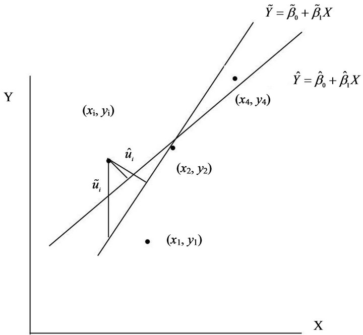
Figure 1. Regression lines obtained from OLS & MPDS method.
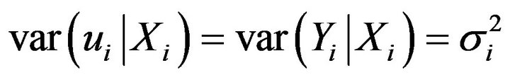
Now if the conditional variance of  are not same for each of the
 . i.e., heteroscedasticity. Symbolically,
and suppose the heteroscedastic variance  are known. Then dividing (1) by
  both sides, we get
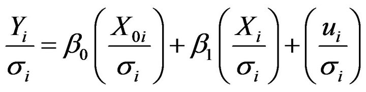 (2)
(2)
which for ease of exposition we write
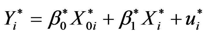 (3)
(3)
where the transformed variables are the original variables divided by (the known) . We use the notation
  and
and , the parameters of the transformed model, to distinguish them from the usual MPDS parameters
  and
and . Now we see
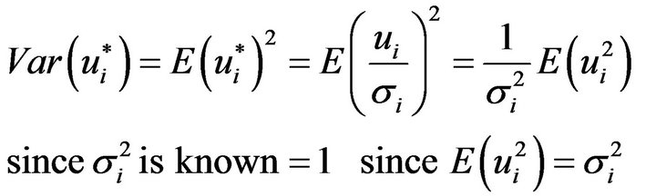
which is a constant. That is, the variance of the transformed disturbance term  is now homoscedastic.
This procedure of transforming the original variables is done in such a way that the transformed variables satisfy the assumptions of the classical model. Now applying MPDS method to this transformed model to estimate parameter we call Generalized Minimum Perpendicular Distance Squares Method (GMPDSM). In short, GMPDS is MPDS on the transformed variables that satisfy the classical regression assumptions. The estimators thus obtained are knows as GMPDSM estimators.
3.1. Perpendicular Distance from the Points to the Line 
Let us consider two-variable linear regression function
Dividing both sides by  we have
 (4)
(4)
or
For estimating  and
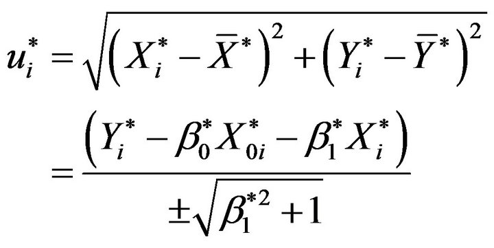
and  we need to determine the perpendicular distance from the observed point
to the line . The perpendicular distance
  from the points
  to the fitted line
 [4,5] is
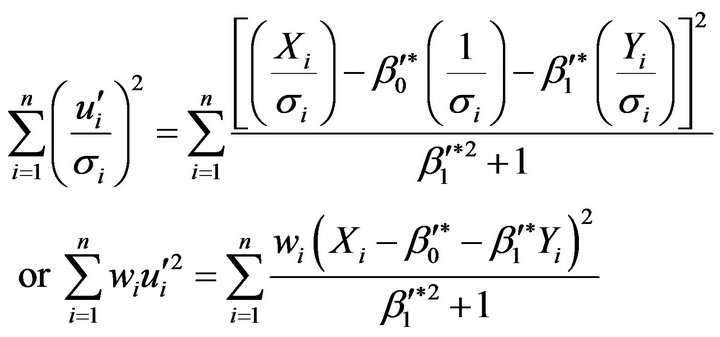
3.2. Parameter Estimation Based on GMPDS Method
To obtain the GMPDS estimators, we minimize sum of square of perpendicular distances  from the points
  to the fitted line
  following steps are taken.
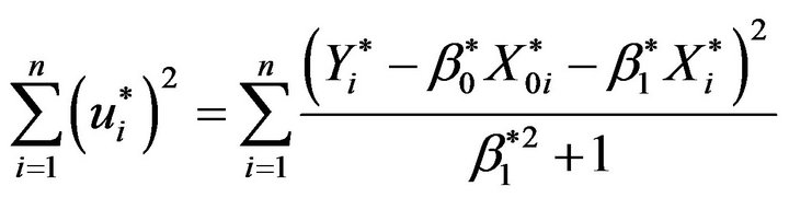
that is,
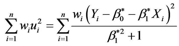 (5)
(5)
where weights
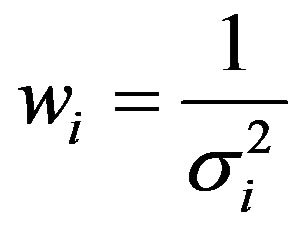
that is, the weights are inversely proportional to the variance of  or
or ![]() conditional on the given
conditional on the given , i.e.,
 .
.
Differentiating (5) with respect to , then putting equal to zero and setting for
 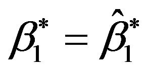 we get the normal equation
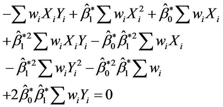 (6)
(6)
Again differentiating Equation (5) with respect to  and equating zero with
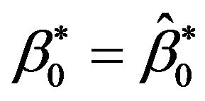 , we get
 (7)
(7)
Using Equation (7) in Equation (6) we get
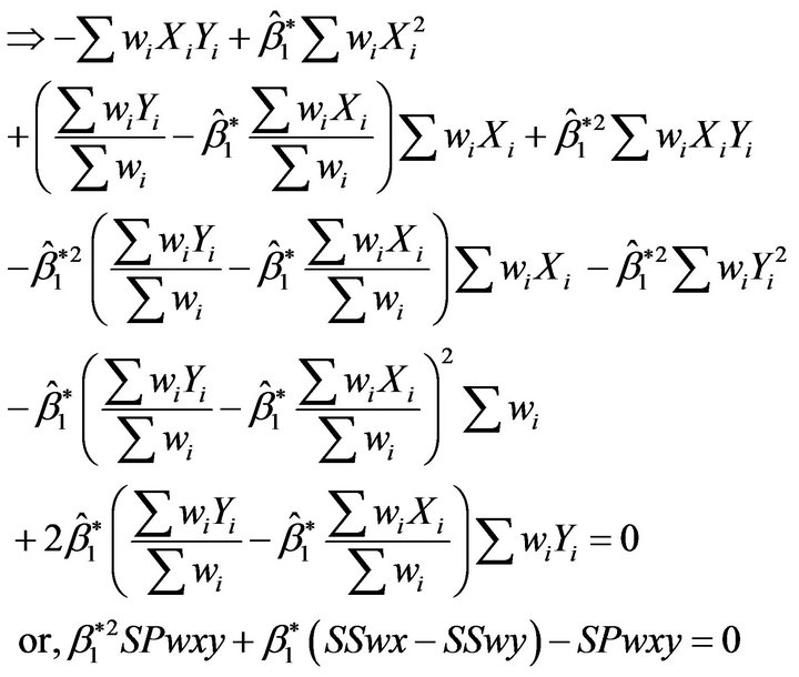
where
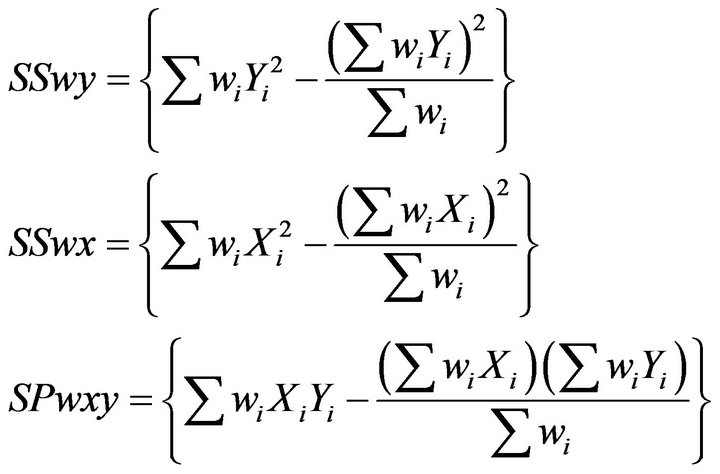
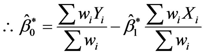
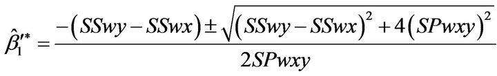
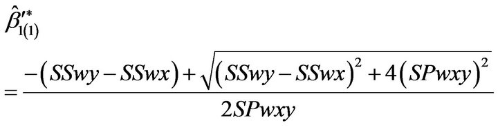
So the solution of the above equation is:
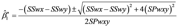
Hence
Using this result in Equation (7) we can estimate . And hence
 (8)
(8)
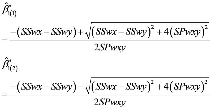
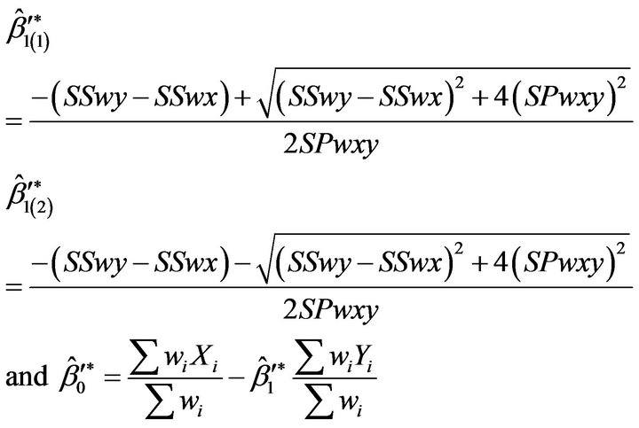
In this method we get two regression coefficients, it could be proved that the “+” solution i.e. ![]() gives minimum of (5) and hence we suggest the reader to use
gives minimum of (5) and hence we suggest the reader to use ![]() as the regression coefficient and accordingly the regression constant
as the regression coefficient and accordingly the regression constant  could be estimated by using
 ![]() in Equation (8) to fit the regression line
in Equation (8) to fit the regression line  on
on  i.e.
i.e. .
.
3.3. Estimation of Regression Coefficient by Using GMPDS for the Model 
To estimate regression coefficient  and regression constant
  by minimizing sum of squares of the error term
 ’s (assumed) the perpendicular distances from the fitted line
 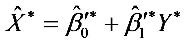 to the points
 ; we do the similar steps as we do in Section 3.7.

That is,
 (9)
(9)
Differentiating both sides with respect to  and
and  and putting equal to zero and setting for
  and
and , we get the following solutions:
Hence
Here we also get two regression coefficients and for the same region as we have mentioned in Section 3.2, we will suggest the reader to use  as regression coefficient and accordingly the estimation of
  may be obtained to fit the regression line
  on
on .
.
3.4. Relationship between Regression Coefficients
If we consider the GMPDS method to estimate regression coefficients  and
and  as we have indicated in Sections 3.2 and 3.3, by minimizing the error term
  and
and  respectively (the perpendicular distances from these lines to the observed points), we get

for the line  and
and
for the line 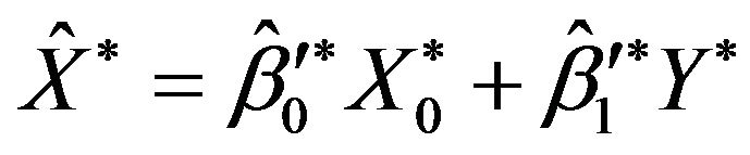 we see that
 ![]() is proportional to
is proportional to ![]() i.e.
i.e.
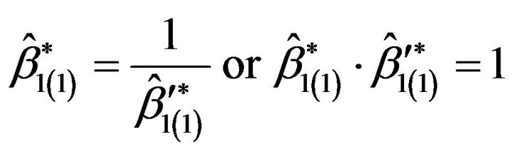 which indicate that during estimating regression coefficient by using GMPDS method in case of heteroscedasticity, the error term is minimized. This is a new angle to advocate the advantage our suggested method (GMPDSM) to estimate regression coefficients in case of heteroscedasticity.
4. Concluding Remarks
The method of MPDS estimation actually minimize real distances from the observed points to the fitted regression line but OLS and GLS method fail to do that by using vertical distance from the observe points to the fitted regression line. But one of the crucial assumptions of MPDS method and also for traditional OLS method is that the variance of each disturbance terms remains some constant number . So we can not apply MPDS method when this assumption is violated. That is, in presence of heteroscedasticity OLS and MPDS is not suitable. In this paper our main focus is on minimum perpendicular deviations in case of heteroscedasticity, and we have shown in mathematically that GMPDS method gives an estimator that the error term is really minimized. Hence we propose GMPDS method in case of heteroscedasticity.
REFERENCES
- W. H. Greene, “Econometric Analysis,” 5th Edition, Pearson Education, Singapore, 2003,
- D. Gujarati, “Basic Econometrics,” 4th Edition, McGraw- Hill, New York, 2003.
- M. F. Hossain and G. Khalaf, “Minimum Perpendicular Distance Square Method Estimation,” Journal of Applied Statistical Science, Vol. 17, No. 2, 2009, pp. 153-180.
- A. Mizrahi and M. Sullivan, “Calculus and Analytic Geometry,” Wadsworth Publishing Company, Beverly, 1986.
- M. R. Spiegel and John Lin, “Mathematical Handbook of Formulas and Tables,” 2nd Edition, Mcgraw-Hill, New York, 1999.