Applied Mathematics
Vol.3 No.8(2012), Article ID:21484,6 pages DOI:10.4236/am.2012.38137
An Efficient Technique for Finding the Eigenvalues of Fourth-Order Sturm-Liouville Problems
Department of Mathematical Sciences, Faculty of Engineering, Mansoura University, Mansoura, Egypt
Email: gamel _eg@yahoo.com
Received June 3, 2012; revised July 10, 2012; accepted July 17, 2012
Keywords: Chebychev Polynomial; Fourth-Order; Sturm-Liouville; Eigenvalue
ABSTRACT
In this work, we present a computational method for solving eigenvalue problems of fourth-order ordinary differential equations which based on the use of Chebychev method. The efficiency of the method is demonstrated by three numerical examples. Comparison results with others will be presented.
1. Introduction
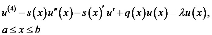
We will apply the Chebyshev method for finding the eigenvalues of the following fourth-order non-singular Sturm-liouville problem:
 (1.1)
(1.1)
where the functions ,
,  ,
,  are in
  and the interval (a,b) is finite. we consider the above equation associated with one of the following pairs of homogenous boundry conditions:
 (1.2)
(1.2)
Numerically, Greenberg and Marletta [1] released a software package, named SLEUTH (Sturm-Liouville Eigenvalues using Theta Matrices), dealing with the computation of eigenvalues of fourth-order Sturm-Liouville problems, which is the only code available in the regard. This situation contrasts with the availability of many software packages dealing with the second-order case, like SLEIGN [2], SLEIGN 2 [3] and SLEGDGE [4].
There is a continued interest in the numerical solution of the fourth-order Sturm-Liouville problems with the aim to improve convergence rates and ease of implementation of different algorithms. Chanane [5,6] introduced a novel series representation for the boundary/ characteristic function associated with fourth-order SturmLiouville problems using the concepts of Fliess series and iterated integrals. The fourth power of zeros of this characteristic function are the eignvalus of the problem. Few examples were provide and the results were in agreement with output of SLEUTH [1]. Chawla [7] presented fourth-order finite-difference method for computing eigenvalues of fourth-order two-point boundary value problems. Usmani and Sakai [8] applied finite difference of order 2 and 4 for computing eigenvalues of a fourthorder. Twizell and Matar [9] developed finite difference method for approximating the eigenvalues of fourth-order boundary value problems Recently, Attili and Lesnic [10] used the Adomian decomposition method (ADM) to solve fourth-order eigenvalue problems. Syam and Siyyam [11] developed a numerical technique for finding the eigenvalues of fourth-order non-singular Sturm-Liouville problems. More recently, Chanane [12] has enlarged the scope of the Extended Sampling Method [13] which was devised initially for second-order Sturm-Liouville problems to fourth-order ones. Abbasbandy and Shirzadi [14] applied the homotopy analysis method (HAM) to numerically approximate the eigenvalues of the second and fourthorder Sturm-Liouville problems. Shi and Cao [15] presented a computational method for solving eigenvalue problems of high-order ordinary differential equations which based on the use of Haar wavelets. Finally, Ycel, and Boubaker [16] applied differential quadrature method (DQM) and boubaker polynomial expansion scheme (BPES) for efficient computation of the eigenvalues of fourth-order Sturm-Liouville problems.
The remaining structure of this article is organized as follows: a brief introduction to the Chebyshev polynomial is presented in Section 2. Section 3 is devoted to the nmerical computation of the eigenvalues of (1.1)-(1.2). Section 4 is devoted to giving some new examples exhibiting the technique. The last section includes our conclusions.
2. Some Properties of Chebyshev Polynomials
In recent years, a lot of attention has been devoted to the study of the Chebychev method to investigate various scientific models. The efficiency of the method has been formally proved by many researchers [17-19]. For more details of the Chebychev method see [20,21] and the references therein. The goal of this section is to recall notation and definitions of the Chebychev function, state some known results, and derive useful formulas that are important for this paper.
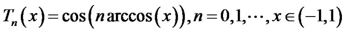
The well known Chebyshev polynomials are defined on the interval [−1, 1] and are obtained by expanding the following formula [20]
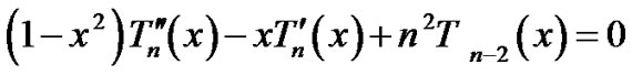
Also they have the following properties a: Three-term recurrence

b: Second order differential equations
c: Orthogonality

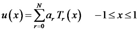
In this paper we use orthonormal Chebyshev polynomials, noting property (c). In the present paper, we are concerned with the approximate solution of (1.1) by means of the Chebyshev polynomials in the form
 (2.1)
(2.1)
where  denotes shifted Chebyshev polynomials of the first kind of degree r, are unknown Chebyshev coefficients and N is chosen any positive integer such that
 . Let us assume that the function u(x) and its derivatives have truncated Chebyshev series expansion of the form
 (2.2)
(2.2)
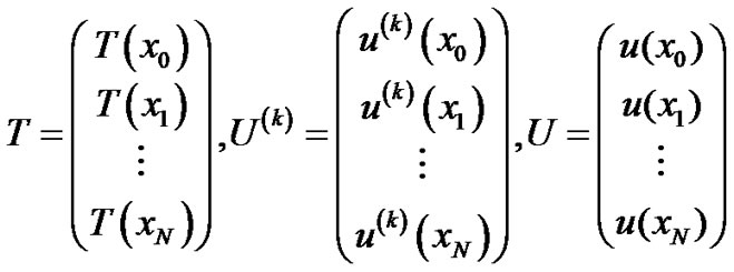
Then the solution expressed by (2.1) and its derivatives can be written in the matrix forms

where
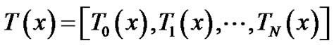 and
and


and
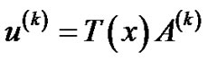
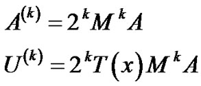
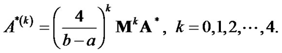
or using the relation between the Chebyshev coefficient matrices  and
and  [21],
[21],
Substituting Chebyshev collocation points defined by
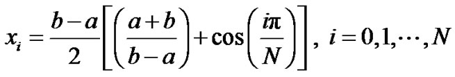 (2.3)
(2.3)
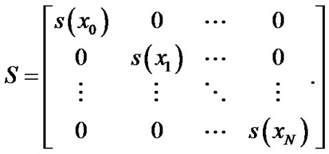
and the matrices are defined as following:
 (2.4)
(2.4)
where
 if N is odd,
 if N is even.
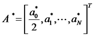
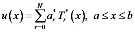
The method can be developed for the problem defined in the domain [a, b] to obtain the solution in terms of shifted Chebyshev polynomials  in the form
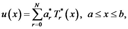
where
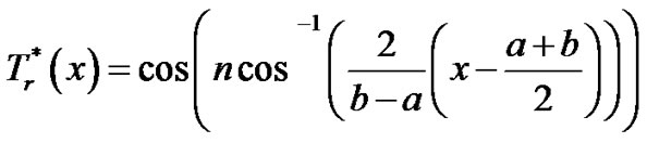 (2.5)
(2.5)
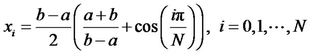
It is followed the previous procedure using the collocation points defined by
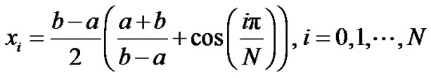 (2.6)
(2.6)
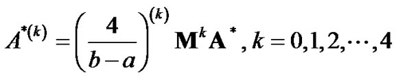
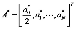
and the relation
where
It is easily obtained , because of the properties of Chebyshev polynomials.
3. The Description of Chebychev Scheme
Consider fourth-order Sturm-Liouville problem of the form
 (3.1)
(3.1)
Let us seek the solution of (3.1) expressed in terms of Chebyshev polynomials as
 (3.2)
(3.2)
It is followed the previous procedure using the collocation points defined by
and the relation
 (3.3)
(3.3)
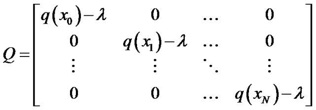
where
Then we obtain the fundamental matrix equation for (3.1) as
 (3.4)
(3.4)
where

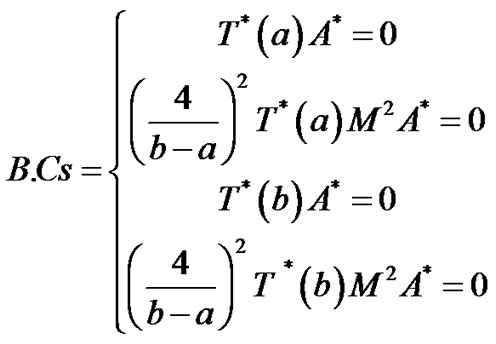
This equation corresponds to a system of N + 1 linear algebraic equations with unknown Chebyshev coefficients . Moreover, the matrix forms of the conditions become Case (1)
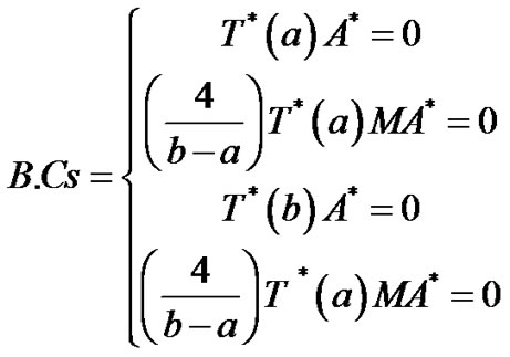
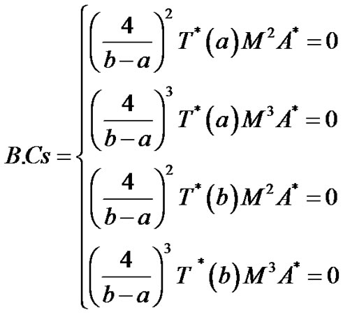
Case (2)
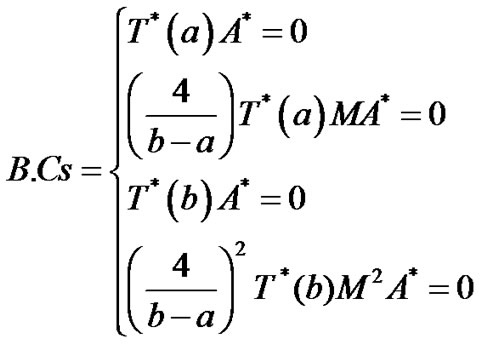
Case (3)
Case (4)
Finally, to obtain the values of eigenvalues of Equation (1.1) under the conditions (1.2), four equations in linear algebraic system (3.4) are replaced with four equations in linear algebraic equations system.
4. Examples and Comparisons
In this section, we will present three of our numerical results of fourth-order Sturm-Liouville problems using the method outlined in the previous section. The performance of the Chebychev method is measured by the relative error  which is defined as
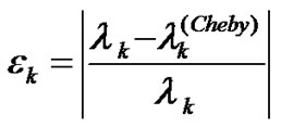
where  indicates k-th algebraic eigenvalues obtained by Chebychev method and
  are the exact eigenvalues.
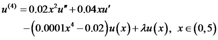
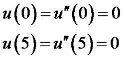
Example 1: [14,16] Consider the eigenvalue problem

and the boundary conditions are given by

The exact eigenvalues in the latter case can be obtained by solving

This analytical solution is commonly available in [16]. Exact eigenvalues, relative error are tabulated in Table 1 for Chebychev method using N = 22 together with the relative error for Differential quadrature method [16].
Table 2 shows the comparison of our results obtained using N = 22, for the first four eigenvalues of the problem with the results of Abbasbandy [14], Syam and Siyyam [11] and Attili and Lesnic [10]. It can be see from Table 2 that our results of Chebychev method are in excellent agreement with the results of [11,14].
Example 2: [10-12,14,16] Consider the eigenvalue problem
and the boundary conditions (simply supported beam) are given by
Example 3: [11] Consider the following fourth-order
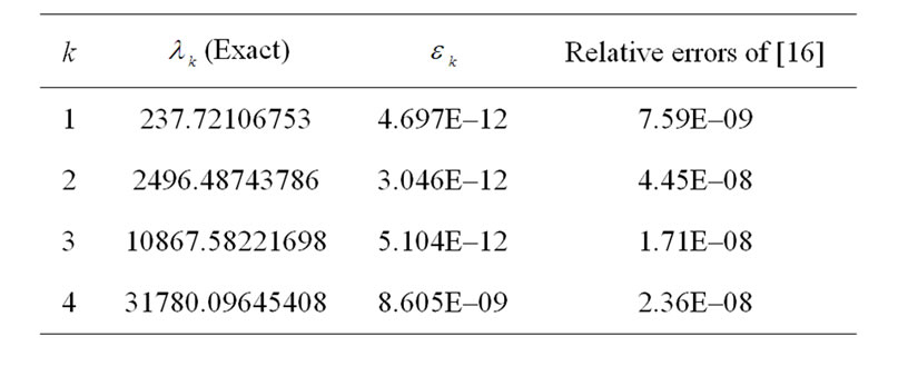
Table 1. Results of Example 1.
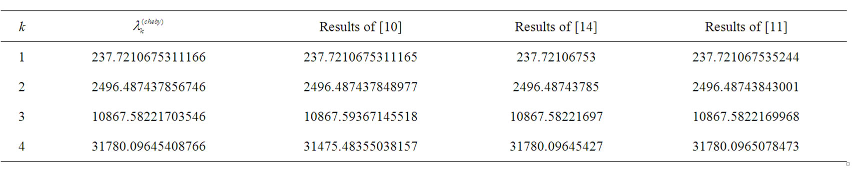
Table 2. Comparison of eigenvalues of Example 1.
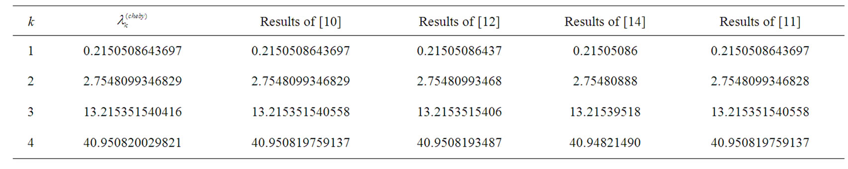
Table 3. Comparison of eigenvalues of Example 2.

Table 4. Eigenvalues of Example 3.
eigenvalue problem

and the boundary conditions are given by


The first three eigenvalues are tabulated in Table 4 for chebychev method using N = 22 together with the analogous results of Syam [11].
5. Conclusion
In this paper, we developed a numerical technique for finding the eigenvalues of fourth-order non-singular Sturm-Liouville problems. To verify the accuracy of the presented technique, we have considered three numerical examples. In the first two examples, we computed the first four eigenvalues and compared our results with other published works in the literature. Excellent agreements are observed between the results of present work and the results of previously published works [10-12,14, 16]. From these comparisons, we see that our results are very close from the results of Syam and Siyyam [11]. Therefore, we conclude that the Chebychev method produces accurate results for the eigenvalues of the fourthorder Sturm-Liouville problems considered in this work. We also suggest the Chebychev method for the numerical solution of the fourth-order problems. Indeed, it will be interesting to see how the method works for the sixth-order Sturm-Liouville problems. This will be considered in a future work.
REFERENCES
- L. Greenberg and M. Marletta, “Algorithm 775: The Code SLEUTH for Solving Fourth-Order Sturm-Liouville Problems,” ACM Transactions on Mathematical Software, Vol. 23, No. 4, 1997, pp. 453-493. doi:10.1145/279232.279231
- P. Bailey, M. Gordon and L. Shampine, “Automatic Solution of the Sturm-Liouville Problem,” ACM Transactions on Mathematical Software, Vol. 4, No. 3, 1978, pp. 193-208. doi:10.1145/355791.355792
- P. Bailey, W. Everitt and A. Zeal, “Computing Eigenvalues of Singular Sturm-Liouville Problems,” Results in Mathematics, Vol. 20, Birkhauser, Basel, 199l.
- C. Fulton and S. Pruess, “Mathematical Software for SturmLiouville Problems,” INSF Final Report for Grants DMS88-13113 and DMS88-00839, Computational Mathematics Division, 1991.
- B. Chanane, “Eigenvalues of Fourth-Order SturmLiouville Problems Using Fliess Series,” Journal of Computational and Applied Mathematics, Vol. 96, No. 2, 1998, pp. 91-97. doi:10.1016/S0377-0427(98)00086-7
- B. Chanane, “Fliess Series Approach to the Computation of the Eigenvalues of Fourth-Order Sturm-Liouville Problems,” Applied Mathematics Letters, Vol. 15, No. 4, 2002, pp. 459-463. doi:10.1016/S0893-9659(01)00159-8
- M. Chawla, “A New Fourth-Order Finite Difference Method for Computing Eigenvalues of Fourth-Order Linear Boundary-Value Problems,” IMA Journal of Numerical Analysis, Vol. 3, No. 3, 1983, pp. 291-293. doi:10.1093/imanum/3.3.291
- R. Usmani and M. Sakai, “Two New Finite Difference Method for Computing Eigenvalues of a Fourth-Order Two-Point Boundary-Value Problems,” International Journal of Mathematics and Mathematical Sciences, Vol. 10, No. 3, 1983, pp. 525-530. doi:10.1155/S0161171287000620
- E. Twizell and S. Matar, “Numerical Methods for Computing the Eigenvalues of Linear Fourth-Order Boundary-Value Problems,” Journal of Computational and Applied Mathematics, Vol. 40, No. 1, 1992, pp. 115-125. doi:10.1016/0377-0427(92)90046-Z
- B. Attili and D. Lesnic, “An Efficient Method for Computing Eigenelements of Sturm-Liouville Fourth-Order Boundary Value Problems,” Applied Mathematics and Computation, Vol. 182, No. 2, 2006, pp. 1247-1254. doi:10.1016/j.amc.2006.05.011
- M. Syam and H. Siyyam, “An Efficient Technique for Finding the Eigenvalues of Fourth-Order Sturm-Liouville Problems,” Chaos, Solitons & Fractals, Vol. 39, No. 2, 2009, pp. 659-665. doi:10.1016/j.chaos.2007.01.105
- B. Chanane, “Accurate Solutions of Fourth Order Sturm-Liouville Problems,” Journal of Computational and Applied Mathematics, Vol. 234, No. 10, 2010, pp. 3064-3071. doi:10.1016/j.cam.2010.04.023
- B. Chanane, “Sturm-Liouville Problems with Parameter Dependent Potential and Boundary Conditions,” Journal of Computational and Applied Mathematics, Vol. 212, No. 2, 2008, pp. 282-290. doi:10.1016/j.cam.2006.12.006
- S. Abbasbandy and A. Shirzadi, “A New Application of the Homotopy Analysis Method: Solving the SturmLiouville Problems,” Communications in Nonlinear Science and Numerical Simulation, Vol. 16, No. 1, 2011, pp. 112-126. doi:10.1016/j.cnsns.2010.04.004
- Z. Shi and Y. Cao, “Application of Haar Wavelet Method to Eigenvalue Problems of High Order Differential Equations,” Applied Mathematical Modelling, Vol. 36, No. 9, 2012, pp. 4020-4026. doi:10.1016/j.apm.2011.11.024
- U. Ycel and K. Boubaker, “Differential Quadrature Method (DQM) and Boubaker Polynomials Expansion Scheme (BPES) for Efficient Computation of the Eigenvalues of Fourth-Order Sturm-Liouville Problems,” Applied Mathematical Modelling, Vol. 36, No. 1, 2012, pp. 158-167. doi:10.1016/j.apm.2011.05.030
- A. Akyȕz and M. Sezer, “A Chebyshev Collocation Method for the Solution Linear Integro Differential Equations,” Journal of Computational Mathematics, Vol. 72, 1999, pp. 491-507.
- H. Ḉerdk-Yaslan and A. Akyȕz-Daciolu, “Chebyshev Polynomial Solution of Nonlinear Fredholm-Volterra Integro-Differential Equations,” Journal of Science and Arts, Vol. 6, 2006, pp. 89-101.
- M. Sezer and M. Kaynak, “Chebyshev Polynomial Solutions of Linear Differential Equations,” International Journal of Mathematical Education in Science and Technology, Vol. 27, No. 4, 1996, pp. 607-611. doi:10.1080/0020739960270414
- T. Rivlin, “An Introduction to the Approximation of Functions,” Dover Publications, Inc., New York, 1969.
- M. Sezer and M. Kaynak, “Chebyshev Polynomial Solutions of Linear Differential Equations,” International Journal of Mathematical Education in Science and Technology, Vol. 27, No. 4, 1996, pp. 607-618. doi:10.1080/0020739960270414