Applied Mathematics
Vol. 3 No. 7 (2012) , Article ID: 19872 , 10 pages DOI:10.4236/am.2012.37116
On the Zeros of Daubechies Orthogonal and Biorthogonal Wavelets*
Faculty of Science and General Studies, Alfaisal University, Riyadh, KSA
Email: jkaram@alfaisal.edu
Received February 3, 2012; revised April 27, 2012; accepted May 4, 2012
Keywords: Orthogonal; Biorthogonal Wavelets; Binomial Polynomials
ABSTRACT
In the last decade, Daubechies’ wavelets have been successfully used in many signal processing paradigms. The construction of these wavelets via two channel perfect reconstruction filter bank requires the identification of necessary conditions that the coefficients of the filters and the roots of binomial polynomials associated with them should exhibit. In this paper, orthogonal and Biorthogonal Daubechies families of wavelets are considered and their filters are derived. In particular, the Biorthogonal wavelets Bior3.5, Bior3.9 and Bior6.8 are examined and the zeros distribution of their polynomials associated filters are located. We also examine the locations of these zeros of the filters associated with the two orthogonal wavelets db6 and db8.
1. Introduction
The Daubechies wavelets construction, requires the finding of a scaling function  and a wavelet function
  [1]. This construction is best described via a two-channel perfect reconstruction filter bank [1,2] and depends on the distribution of the zeros of some polynomials in the plane. The literature provides many theorems describing geometric locations of the roots of certain polynomials [3,4]. Identifying necessary conditions for the coefficients of the filters associated with the construction is vital for orthogonality, Biorthogonality and alias cancellation. The distribution of the zeros of the binomial polynomial related to the construction of these wavelets were proved to reside inside the unit circle [5], and better limits for these roots based on a generalization of the Kakeya-Enestrom Theorem were derived in [6] where it was shown that if y is a root of a binomial polynomial of degree
 , then:
 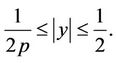 A subclass of polynomials is derived from this construction process by considering the ratios of consecutive binomial polynomials’ coefficients essentials to these constructions. We showed mathematically that the roots of this class of polynomials reside inside the unit circle. In Section 3, the construction of Daubechies orthogonal wavelets is detailed. In Section 4, the new class of polynomials is introduced and the distribution of their zeros is examined and mathematically shown to reside inside the unit circle. An example is then presented illustrating the location for the zeros of the derived polynomial of the orthogonal mother wavelet db6. The case of db8 is then examined in Section 5 and results are obtained. Section 6 describe the conclusion of this work.
2. Related Works
A two-channel filter bank has a low-pass and a high-pass filter in the decomposition (analysis) phase and anotherlow-pass and a high-pass filter in the reconstruction (synthesis) phase. Let  and
and  denote the low-pass filter coefficients and the high-pass filter coefficients respectively of the analysis phase, then given the coefficients of
 , it is shown in [1,7] that the coefficients of the filters
 ,
,  and
and  that lead to orthogonality can easily be derived from the coefficients of
 . Therefore, to construct a Daubechies orthogonal wavelet, all we need to do is to find the coefficients of the filters
  associated with it.
The distribution of the zeros of a family of polynomials having their coefficients as the ratios of those of the binomial polynomials is considered in Section 4 and proved to reside inside the unit circle. Similar discussions about Daubechies’ Biorthogonal wavelets family are also included along with the constructions of Bior3.5, Bior3.9 and Bior6.8. In the orthogonal case, the scaling and wavelet functions are derived from the coefficients of the filters ,
,  ,
,  and
and . They must satisfy respectively the following two equations [1]:
 (1)
(1)
 (2)
(2)
Biorthogonal filter banks produce Biorthogonal wavelets. This calls for a new scaling function  and a new wavelet function
 . Here, one needs the following conditions:
  and
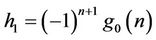
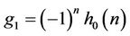
and  [8]. The wavelet filters for analysis banks are derived [1] from the scaling filters using the two relations:
 (3)
(3)
 (4)
(4)
The analysis scaling and wavelet equations thus become:
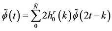 (5)
(5)
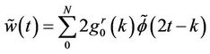 (6)
(6)
where  and
and  are the reverse of the original filters h0 and g0 respectively. The construction of
 ,
,  ,
,  and
and  starts with imposing the Biorthogonality conditions on the filters. The lowpass analysis coefficients
  are the product of a double shift Biorthogonal to the lowpass synthesis coefficients
 :
:
 (7)
(7)
 (8)
(8)
And the highpass filter is Biorthogonal to the lowpass filter:
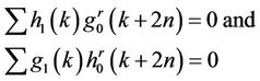 (9)
(9)
Figure 1 shows the frequency responses of the decomposition and reconstruction filters and, the decomposition and reconstruction scaling and wavelet functions of the Biorthogonal (Bior3.9) [9]. Figure 2 shows this Biorthogonl wavelet zeros’ distribution of its decomposition and reconstruction filters. This wavelet possesses the propreties of being smooth with a linear phase and short length filters. Also, Table 1 displays the coefficients of the low-passes and high-passes filters of Bior3.9. Figure 3 and Figure 4 show the zeros’ distributions for the filters associated with Bior6.8 and Bior3.5 respectively.
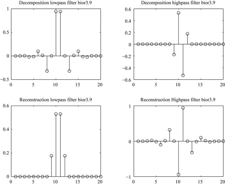
Figure 1. Bior3.9 impulse response for the decomposition and reconstruction filters.
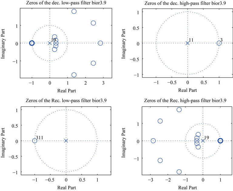
Figure 2. Bior3.9 zeros distribution of the decomposition and reconstruction filters.
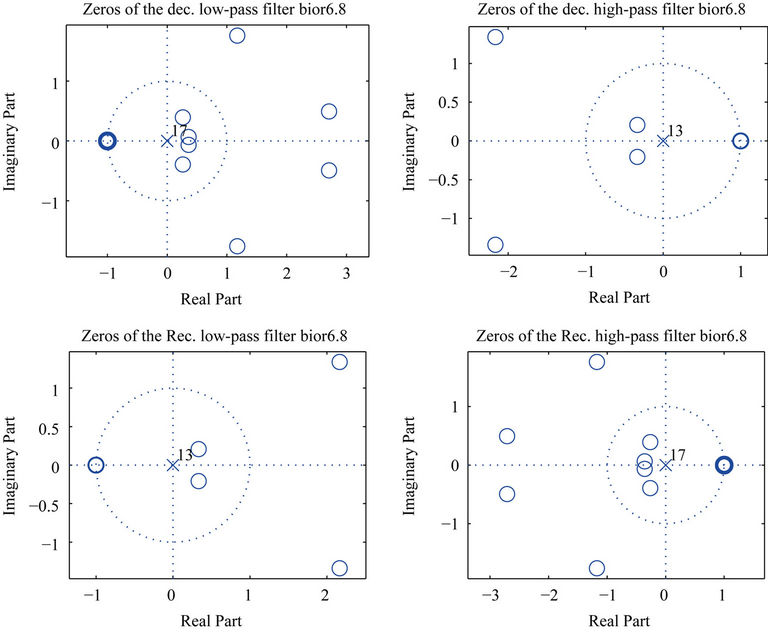
Figure 3. Bior6.8 zeros distribution of the decomposition and reconstruction filters.
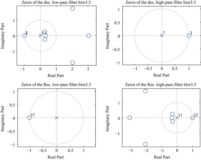
Figure 4. Bior3.5 zeros distribution of the decomposition and reconstruction filter.
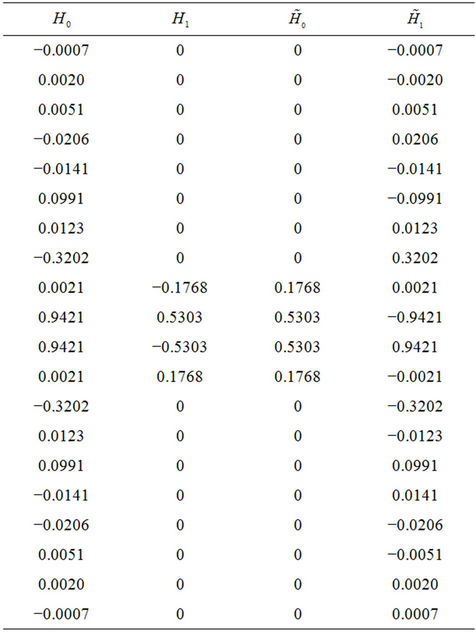
Table 1. Filter coefficients of the biorthogonal wavelet Bior3.9.
3. Construction of Daubechies Orthogonal Wavelets
Wavelets such as db6 and db8 have played a very essential role in a variety of speech recognition and compression paradigms introduced last decade [10,11]. The low-pass and high-pass filters in the decomposition phase of a two channel filter bank are depicted in Figure 5 and two more filters of the reconstruction phase are displayed in Figure 6.
Let  and
and  denote the low-pass filter coefficients and the high-pass filter coefficients respectively in the analysis phase. To obtain perfect reconstruction, these two filters must satisfy the following conditions [1,2]:
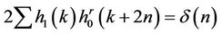
1) For the low-pass filter :
:
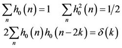 (10)
(10)
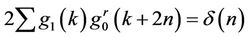
2) For the high-pass filter :
:
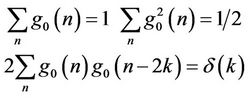 (11)
(11)
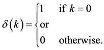
where  is the Dirac delta function defined by:
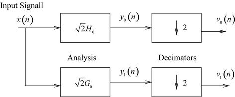
Figure 5. Analysis phase filters of a two-channels filter bank.
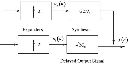
Figure 6. Synthesis phase filters of a two-channels filter bank.
Given the coefficients of , it is shown in [1,7] that the coefficients of the filters
 ,
,  and
and  that lead to orthogonality can easily be derived from the coefficients of
 . Therefore, to construct a Daubechies orthogonal wavelet, all we need to do, is to find the coefficients of the filter
  associated with it.
The construction of the filter bank amounts to [1]:
1) Design a product low-pass filter  satisfying:
 (12)
(12)
2) Factor  in
in , then find
  and
and . And can be reduced even further by defining:
  and substituting
  by
by . Hence, the perfect reconstruction condition becomes [8]:
 (13)
(13)
which implies that  is a half band filter [1] with all of its the coefficients zeros except the constant term 1. Furthermore, the odd powers cancel when we add
  to
to . The design of the low-pass and the high-pass filters of the synthesis and analysis filter banks of a Daubechies orthogonal wavelet, considers the following two properties [1]:
1) These wavelets filters must be orthogonal.
2) And must have maximum flatness at  and
and  in their frequency responses.
The low-pass filters will have p zeros at , and have a total of 2p coefficients, (length of the filters). This filter bank is orthogonal and the product filters
  and
and  have a length of
 . The construction of Daubechies orthogonal wavelets begins by choosing the number of zeros p at
 . The zeros the filters associated with the db6 are depicted in Figure 7. Here, we also need to choose the binomial polynomial
  associated with it which has a degree of
  The coefficients of these polynomials can be found recursively for p by using the following equation:
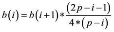 (14)
(14)
For a given value p, the coefficients of  are in an ascending order [5]. To get the roots of
 , one scales b by 4 and to facilitate the numerical calculations, one uses the variable 4y instead of y. The ratio of any two consecutive coefficients is:
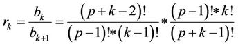 (15)
(15)
Which in its simplest form can be expressed as:
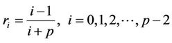 (16)
(16)
This equation will be used in Section 5 to construct the family of polynomials with coefficients equal to the ratios of this polynomial consecutive coefficients.
Now to compute the  zeros of
  other than −1, we note that according to [1,9] the frequency response of the half-band filter
  is given by:
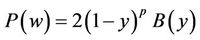
where  or
or .
.
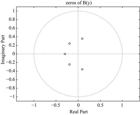
Figure 7. Zeros of B(y) for db6.
On the unit circle we have:
 .
.
Also, off the unit circle we use the same relation between z and y. Rearranging these terms leads to:
 (17)
(17)
Now let  and
and  then,
then,
with , this implies that:

and

are the two roots of  for each root y of
 .
.
Note that .
.
That is, we have  roots and their inverses, namely:
and

and
 .
.
The distribution of these zeros in the plane is shown in Figure 8. From ,
,  is then derived and all is left is to factorize
 . Daubechies did the following factorization found in [1]:
 (18)
(18)
where  is a polynomial of degree
 .
.
The Construction of db6
For p = 6, the db6 wavelet is obtained. Figure 8 shows the location in the complex plane for the zeros of  associated with the Daubechies db6 orthogonal wavelet. The frequency responses of the analysis lowpass filter
  and synthesis lowpass filter
  of this wavelet are depicted in Figure 9. Therefore completing the construction of the scaling function along with the mother wavelet. The decomposition and reconstruction functions for the mother wavelet db6 are plotted in Figure 9, while Figure 10 shows the impulse response of the four filters associated with it.
Now, given the coefficients  of the low-pass filter
 , it is shown in [1,7] that the coefficients of the filters
 ,
,  and
and  that
that
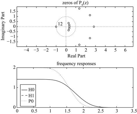
Figure 8. Zeros of P(z) for db6 and the frequency responses of the filters P, H0 and H1.
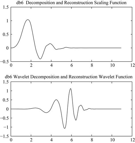
Figure 9. The db6 analysis and synthesis scaling and wavelet functions.
lead to orthogonality can be derived from the coefficients of  as follows:
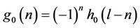
First, the coefficients of the high-pass filter  of the analysis bank are obtained from those of the low-pass filter
  by the “alternating flip”.
This can be represented by three operations on the coefficients of .
.
1) Reverse the order;
2) Alternate the signs;
3) Shift by an odd number l.
This takes the low-pass filter coefficients into an orthogonal high-pass filter [1] which is represented in the
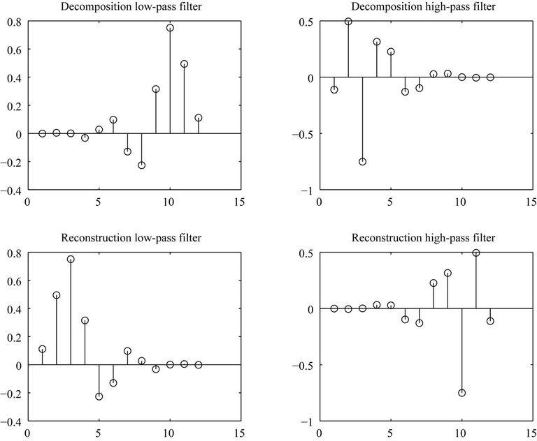
Figure 10. Impulse response for the reconstruction and decomposition filters of db6.
following equation:
 (19)
(19)
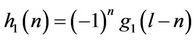
Then, the coefficients of the high-pass filter  of the synthesis bank are obtained by the reverse of the coefficients of the high-pass filter
  of the analysis bank. They can be generated by the following equation:
 (20)
(20)
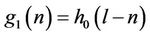
The coefficients of the low-pass filter  of the synthesis bank are the alternating flip of the coefficients of
 . They can be generated by the following equation:
 (21)
(21)
where l is the length of the low-pass filter  [1].
[1].
The scaling and wavelet functions are then derived from the coefficients of these filters. The scaling function satisfies the equation [1]:
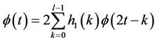 (22)
(22)
where,  is the reverse of
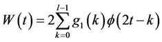
  and the wavelet function is then derived from the scaling function by the equation:
 (23)
(23)
4. Zeros of Ratio Coefficients Polynomials
Now we consider the class of polynomials with coefficients those of the ratios obtained in Equation (4). An optimal limit of these zeros in the complex plane was presented in [12]. Other theorems and alternative approach to proving this distribution can be found in [13]. Now the rations can be expressed as follows:
We note that these coefficients are in an ascending order where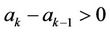 .
.
Theorem I: The roots of the polynomials  lie inside the unit disk for all p.
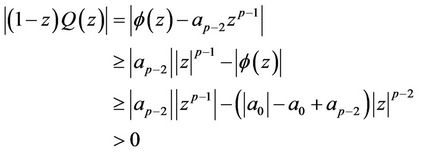
Proof: For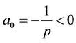 , consider
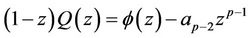
where
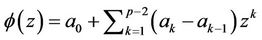 .
.
For , we have:
 .
.
Now for ,
,
and
 .
.
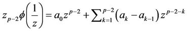
Replacing z with , we get:
 for
for .
.
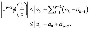
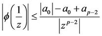
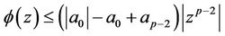
Hence, if 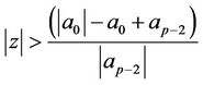 (i.e.
(i.e. ), then:
The Distributions of Zeros for db6
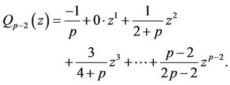
For the Daubechies wavelet “db6” this polynomial is:

with maximum module of 0.9325. The roots of this polynomial are depicted below in Figure 11 and observed to reside all in the unit circle.
5. The Construction of db8 The scaling and wavelet functions are then derived from the coefficients of these filters. They satisfy respectively the equations [1]:
 (24)
(24)
 (25)
(25)
To compute the 14 zeros of  other than −1, note that on and off the unit circle we have the following relation between z and y:
 . This implies that the equation:
 (26)
(26)
The coefficients of  are displayed in Table 2.
If one sets  and
and  then, z = x + u and
  are the two roots of
  for each root y of
 . Note that
 . That is, we have 7 roots and their inverses, The plot of these zeros in the plane are shown in Figure 12. Also, the values of
 ,
,  and
and  are listed in Table 3.
From the definition of ,
,  is obtained and all is left now is to factorize
 . Were
  is a polynomial of degree 14 and chosen to satisfy Equation 16. It is equal to
 . The different factorizations of
  into
into  lead to different mother wavelets. Choosing
  to have its seven zeros inside the unit circle and
  to have its seven zeros outside the unit circle leads to the Daubechies orthogonal mother wavelet db8.
The scaling and wavelet functions of one of the Daubechies wavelets’ family member called db8 are shown in Figure 13. The same figure also shows the impulse response of the four filters associated with that wavelet and Table 4 displays The coefficients of the of db8 filters.
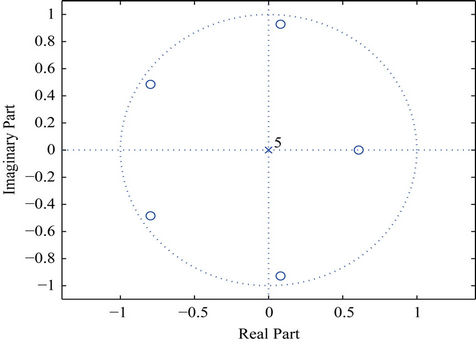
Figure 11. Zeros of Q4(z) for Daubechies db6 orthogonal wavelet.
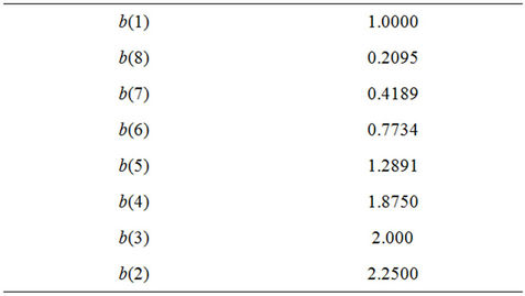
Table 2. The coefficients of the polynomial B8(y).
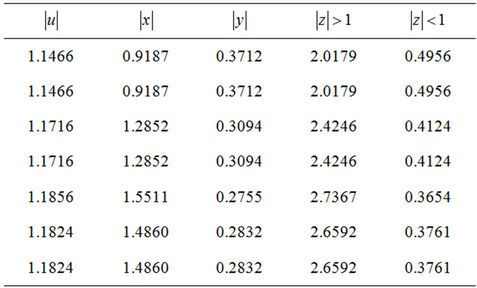
Table 3. The roots of Q14(z) inside the unit circle z = x – u and outside of it z = x + u.
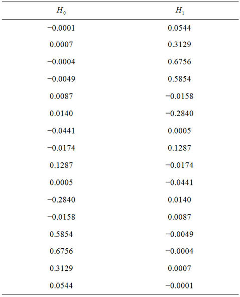
Table 4. The coefficients of the of db8 filters.
To carry out the factorization we note that  has 16 roots at
  and 14 other roots which occur in pairs (z and
 ). This means that we have 7 roots inside the unit circle and the other 7 roots outside the unit circle. The roots inside the circle are the roots for the filter
  coming from the equation:
  and the ones outside it are for filter
  obtained from the equation:
 . These roots when factorized lead to the coefficients of these two filters and they are shown in Table 3 for
 . The coefficients of the high-pass filters
  and
and  are simply then derived from the low-pass filter coefficients by the alternating sign property.
The scaling and wavelet functions of one of the
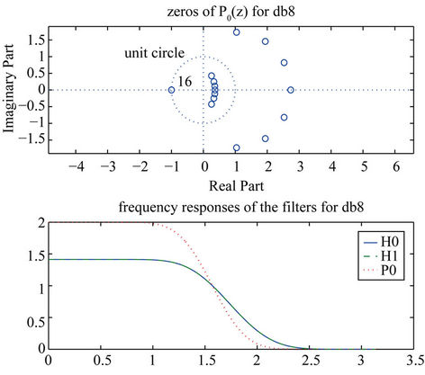
Figure 12. Zeros of P(z) for db8 and the frequency responses of the filters: P0, H0 and H1.
Daubechies wavelets’ family member called db8 are shown in Figure 13. The same figure also shows the impulse response of the four filters associated with that wavelet.
The general characteristics of this wavelet include compact support for which exact reconstruction are possible with FIR filters. Its associated scaling filter is a minimum-phase filter. This wavelet is a member of the orthogonal set of wavelets that are usually denoted by:  N represents the order of the reconstruction and decomposition wavelet. Their corresponding filter length is
 .
.
6. Conclusion
In this paper we construct Daubechies orthogonal wavelets via the two channel perfect reconstruction filter bank. The cases of db6 and db8 are examined where we derived the coefficients of the filters associated with these wavelets and the roots of the binomial polynomials that made this construction possible. The locations of the zeros of the polynomials involved in this construction were found and their locations were discussed. The distribution of the zeros of a family of polynomials having their coefficients as the ratios of those of the binomial polynomials was examined and were proved to reside inside the unit circle. Similar discussions about the Daubechies Biorthogonal wavelets family are included along with the constructions of Bior3.5, Bior3.9 and Bior6.8.
7. Acknowledgements
The author would like to thank Alfaisal University and its Office of Research for securing the time, environment and funds to complete this research project. This work
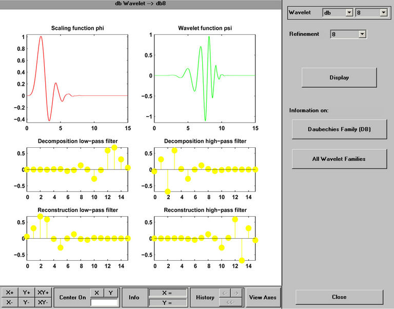
Figure 13. db8 Wavelet and scaling functions. The impulse response for the reconstruction and decomposition filters of the wavelet db8.
was also supported by the Alfaisal University Start-Up Fund (No. 410111410091).
REFERENCES
- G. Strang, and T. Nguyen, “Wavelets and Filter Banks,” Wellesley-Cambridge Press, Wellesley, 1996.
- I. Daubechies, “Ten Lectures on Wavelets,” SIAM, Philadelphia, 1992.
- S. Kakeya, “On the Limits of the Roots of an Algebraic Equation with Positive Coefficients,” Tohoku Mathematical Journal, Vol. 2, 1912, pp. 140-142.
- J. Karam, “On the Kakeya-Enestrom Theorem,” MSc. Thesis, Dalhousie University, Halifax, 1995.
- J. Karam, “Connecting Daubechies Wavelets with the Kakeya-Enestrom Theorem,” International Journal of Applied Mathematics, Vol. 14, No. 2, 2003, pp. 109-124.
- J. Karam, “On the Roots of Daubechies Polynomials,” International Journal of Applied Mathematics, Vol. 20, No. 8, 2007, pp. 1069-1076.
- M. Vetterli, “Wavelets and Filter Banks: Theory and Design,” IEEE Transactions on Signal Processing, Vol. 40, No. 9, 1992, pp. 2207-2232. doi:10.1109/78.157221
- M. Vetterli and J. Kovacevic, “Wavelets and Suband Coding,” Prentice Hall, Englewood Cliffs, 1995.
- M. Misiti, Y. Misiti, G. Oppenheim and J. Poggi, “Matlab Wavelet Tool Box,” 1997.
- J. Karam, “A Comprehensive Approach for Speech Related Multimedia Applications,” WSEAS Transactions on Signal Processing, Vol. 6, No. 1, 2010, pp. 12-21.
- J. Karam, “Radial Basis Functions With Wavelet Packets For Recognizing Arabic Speech,” The 9th WSEAS International Conference on Circuits, Systems, Electronics, Control and Signal Processing, Athens, December 2010, pp. 34-39.
- J. Karam, “On the Distribution of Zeros for Daubechies Orthogonal Wavelets and Associated Polynomials,” 15th WSEAS International Conference on Applied Mathematics, Athens, 29-31 December 2010, pp. 101-105.
- C. A. Muresan, “Comparative Methods for the Polynomial Isolation,” Proceedings of the 13th WSEAS International Conference on Computers, 2009, pp. 634-638.
NOTES
*Dedication: This paper is dedicated to my professors and supervisors Karl Dilcher and William Phillips.