Modern Economy
Vol.07 No.05(2016), Article ID:67012,21 pages
10.4236/me.2016.75071
Economic Inequality among US Farm Households: Assessment of the Role of the 2008-2009 Financial Crisis*
Hisham S. El-Osta, Ron L. Durst
Economic Research Service, Washington DC, USA

Copyright © 2016 by authors and Scientific Research Publishing Inc.
This work is licensed under the Creative Commons Attribution International License (CC BY).
http://creativecommons.org/licenses/by/4.0/


Received 12 April 2016; accepted 28 May 2016; published 31 May 2016
ABSTRACT
This paper aims to evaluate the potential impact of the 2008-2009 financial crisis on the economic inequality among US farm households. To accomplish this objective, a multivariate regression procedure and a decade-long pooled state-level cross sections of data from the Agricultural Resource Management Survey (ARMS) were used. Among the major findings is the inverse relationship between both income and wealth inequality and factors such as when the famer has a college education or beyond, when the farm is owned partly or fully, and when the farm is located in the Midwestern region. These findings underscore the importance, in terms of policy perspectives aimed at lowering economic inequality, of investing in human capital and in maintaining a stable agricultural economy.
Keywords:
Economic Inequality, Financial Crisis, ARMS, Shapley Value

In 1933, and as a consequence of The Great Depression of 1929 that adversely impacted the economic well-being of all Americans, farm households in particular seem to have suffered the worst in terms of economic contraction as rural incomes were 40 percent lower than urban incomes [1] . Historically, and because of relevance to farm policy which has focused since the 1930s on stabilizing farm household income at levels that are “equitable” compared to incomes of nonfarm households, most attention by economists has focused on farm income [2] - [7] .
Consideration of the income generation capacity and wealth accumulation and of their size distributions, as has been noted by Mishra et al. [8] ; among others, is important since both income and wealth affect the economic well-being of the farm households. While income provides the means of livelihood and growth in the standard of living, wealth affects the production of agricultural goods and enables farm households to secure credit, facilitate inter-generational transfer, and smooth consumption expenditures in times of temporary income shortfalls [9] - [11] . A case in point of the importance of wealth, with its relevance to farm households’ well-being, is the study by Gittleman and Wolff [12] that points to a view among researchers and policymakers that began to gain support since the late 1980s that US poverty policy could only be effective if a narrowing in the gap between the asset rich and the asset poor is achieved. Policy analysts, farm investors, and lenders are among those interested in monitoring and forecasting the economic well-being of the farm sector and farm households based on both income and wealth measures.
The financial crisis of 2008-2009 has caused major adverse economic consequences in the US and across the world economy [13] [14] . Since 2008, the weakening in commodity demand has led to increased unemployment rates and reduced economic growth1. The purpose of this research is to evaluate the potential impact of this financial crisis on the economic inequality among US farm households. To accomplish this objective, a multivariate regression procedure and a decade-long pooled state-level cross sections of data from the Agricultural Resource Management Survey (ARMS) were used. In doing so, and in utilizing a regression-based decomposition technique, this paper has allowed for the discernment of the role that certain demographic, economic, and locational factors, among others, play in impacting the inequality in income and wealth measures among US farm households. In the case of farm household income where the dominant income source is from off-farm wages and salaries, and since offered wages and hiring decisions are tied to the stock of knowledge of individuals seeking employment and to the health of the local economy [16] [17] , controlling for both demographic and macro-economic factors when examining economic disparity becomes evident.
Figure 1 provides a cursory look at the extent of rising inequality over the time period considered by depicting the ratio of the income and wealth at the top 1 percentile levels of the income and wealth distributions of farm households relative to their corresponding median levels. While the income and wealth levels at the top 1 percentiles of the distributions were at around 9 times their corresponding median levels in 2003, they were at around 14 times the income and the wealth levels of the median farm household in 2012, with income exhibiting an even larger spike in disparity than wealth just prior to the financial crash of 2008.
Understanding how much of total inequality in income and wealth is attributed to the factors considered will inform the debate among policymakers and researchers alike, considering its relevance to taxation and social welfare [18] [19] and on how inequality concerns among farm households could be mitigated. A case in point is the role farm program payments play in increasing farm households’ income, this in addition to their capacity in increasing households’ net worth as a result of the capitalization of payments into land values, and in increasing savings and investments [20] - [22] . In carrying the analysis out on a state-level basis, this will provide information for policymakers who are considering targeting safety-net and regional development programs to the states where the income and wealth gaps among poorer and richer households are the widest. A delineation of such states is provided in Figure 2 which shows both median incomes and wealth of farm households in eighteen states, primarily in the South, to be lower than both medians when measured across all of the lower forty-eight states and over the decade-long timeframe considered in the analysis.
1. Literature Review
The literature on the disparity in the distributions of income and wealth and how to measure it, because of relevance to social welfare, continues to grow, not just in the US, but in many countries around the world. Aristei and Perugini [23] , for example, allowed for the use of country-specific parameters of inequality aversion from 26 European countries in order to account for the heterogeneity in social preferences in the design and assessment of redistributive policies. Allanson [24] , El Benni and Finger [25] , and Severini and Tantari [26] , among others, have utilized inequality-based approaches to assess the redistributive effect of agricultural policy in a number of European countries. Gradin and Rossi [27] and Araar [28] utilized kernel densities and polarization summary indices to examine, respectively, the changes in the shape of the distribution of income in Uruguay after

Figure 1. Ratio of the top 1 percent (P99) income and wealth levels to the corresponding medians (P50) of farm households: 2003-2012.

Figure 2. Status of median income and wealth ($2012) of farm households by state relative to corresponding national median levels: 2003-2012.
the late eighties and in Canada between 1993 and 2005. Examples of yet other research with a broader economic and statistical implementation of the concept of inequality as it relates to underlying theoretical and welfare-based assumptions (e.g., savings, inheritance policies, labor heterogeneity, effects of population and economic growth, human and nonhuman capital; quality of life, long run development of income and wealth distributions, etc.) with references to the population at large are those by [29] - [38] .
Reinsel [39] , Larson and Carlin [40] , and Ahearn et al. [41] were among the early researchers in the US to have assessed the extent of disparity in the size distributions of income and/or wealth of farm households. Findeis and Reddy [42] have measured the inequality in the distribution of income for farm families, by region, using the 1995 Current Population Survey. Gould and Saupe [43] have assessed the disparity of a combined income and wealth measure for farmers using Wisconsin panel data. Weldon, Moss, and Erickson [44] , and Mishra, Moss, and Erickson [11] examined the changes in United States’ farm wealth over a three-decade period using both state-level and national-level data. Their findings point to the importance of factors such as farm income, government program payments, and income from off-farm employment in generating a more equitable wealth distribution. Mishra, Moss, and Erickson [45] used an entropy-based measure along with multi-year farm level data to examine the inequality in the distribution of farm wealth within-states and between-states in the US. Findings from the study showed that the observed reduction in farm wealth inequality is attributed to increased equality in the distribution of real estate assets of the farm households, which comprise the major component of total farm wealth. Katchova [22] examined the inequality in the distributions of income and wealth using national datasets for farm and nonfarm households. Findings from the study showed nearly similar levels of income inequality among the two groups of households but a higher level of wealth disparity among non-farm households. El-Osta et al. [46] , Mishra, El-Osta, and Shaik [47] , and Mishra, El-Osta, and Gillespie [48] have extended the previous studies by exploring specifically the impact of government payments and off-farm work on income inequality using national survey-based datasets. Other studies by El-Osta and Morehart [49] and by El-Osta and Mishra [50] have examined using also national survey-based datasets the role of value judgments concerning society’s level of aversion to wealth concentration and of farm subsidies on wealth dispersion among farm households.
2. Data
The main data source for this research is the 2003-2012 ARMS. The ARMS, which has a complex stratified, multi-frame design, is a national survey conducted annually by the National Agricultural Statistics Service (NASS) and the Economic Research Service2. Each observation in the ARMS represents a number of similar farms (e.g., based on land use, size of farm, etc.), the particular number being the survey expansion factor (or the inverse of the probability of the surveyed farm being selected for surveying), and is referred to henceforth as survey weight, or wi (i = 1, ∙∙∙, n, where n denotes sample size). In using these weights, the expanded population of farm households in any of the years considered stands at around 2.1 million.
Because some of the states in some of the years were too small to allow for statistical precision of estimates (i.e., 30 observations or less), eight states out of the forty-eight lower states were combined into one geographic category; “other”3. Summary statistics of indicators of income and wealth inequality and of factors perceived to impact these separate indicators are then computed over the 410 state/year observations.
3. Inequality Analysis
“Adjusted” Gini Coefficient
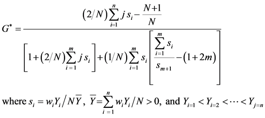
This method of measuring inequality was developed originally by Chen, Tsaur, and Rhai [51] and was further developed by Berrebi and Silber [52] . Unlike in the case of the “standard” Gini coefficient, the “adjusted” Gini coefficient (G*) corrects the problems associated with the presence of negative observations, which are prevalent in the data that were used, by normalizing the distribution of Yin a manner so that the upper bound on the Gini coefficient is unity4. The “adjusted” Gini coefficient is computed on a national (except for Alaska and Hawaii) and on a state-level basis over the 2003-2012 periods as:
 (1)
(1)
In this equation, and for each of the time periods, wi is the survey weight of the ith household in the state, n and N are, respectively, the sample size and the expanded number of farm operator households in the state, si is the corresponding weighted income share of the ith household in the state, Yi is the household’s total income (or total wealth) in the state where  with some Yi< 0, and m is the size of the subset of the households whose combined weighted income is zero with
 . For computational purposes, m is determined where the sum of incomes over the first m households is negative and the first m + 1 household is positive.
Prior to implementing the measurement of inequality, Yi is divided by the square root of household size in order to allow, without differentiation between adults and children, for certain level of economies of scale [54] [55] 5. The implication of this equivalised notion of Y is that a household’s economic requirements increase less than proportionally with its size; e.g., the needs for a family of four persons are twice as great as those of a single person household [56] .
4. What Drives Income and Wealth Inequality?
4.1. Theoretical Consideration
The choice of the variables in the regression models used to attend to this question was based primarily on the human capital and the life-cycle theories due to their relevance to the size distribution of both income and wealth6. The central thesis of the human capital-based theory is that investment in skill through formal education and/or through experience acquired through on-the-job training is rewarded in the labor market, because of enhanced productivity of workers, through higher earnings. The most consistent literature on the relationship between human capital development and the potential for higher earnings dates back to the early work of Friedman and Kuznets [58] and a few decades later, among others, to Mincer [59] [60] , Becker and Chiswick [61] , Ben-Porath [62] , Ritzen and Winkler [63] , Becker [64] - [67] , and Wilson [68] . As for the life-cycle theory as originally developed by Modigliani and Brumberg [69] and as was later extended by Ando and Modigliani [70] to allow for macroeconomic implications, its main focus is the delineation of the consumption and saving patterns of individuals over the course of their life-cycle which involves accumulation of assets in the early stages of life and a dissaving behavior after retirement.
The need for incorporating human capital and life-cycle effects when examining the size distribution of farm income and wealth is rooted in their potential impact on the income generation and wealth accumulation capacity by farmers. Studies by Schultz [71] [72] and Nelson and Phelps [73] , among others, posited that education may enhance farmer’s innovative ability thereby facilitating the diffusion of new technology, a premise that was later demonstrated by the pioneering work by Huffman who also explored the linkages between human capital, race, and off-farm work decisions [74] - [78] 7. Similarly, the importance of the stage in the life cycle of farmers to production agriculture has been documented in many studies. For example, because older farmers have a shorter planning horizon and are more averse to risk than young farmers, they tend to be less inclined to adopt new technology or to purchase newer equipment [80] - [82] than their younger counterparts. As a result, the current market value attached to the existing physical capital of older farmers tends to be lower than that of younger farmers.
4.2. Empirical Estimation
The factors that may explain state-level inequality in income or wealth of farm households over the time period considered (state = 1, ∙∙∙, 41; t = 1, ∙∙∙, 10) are identified by estimating a weighted least squares (WLS) regression model. Since the values of  are between 0 and 1, fitting a linear probability model on
  could result in predictions outside the unit interval. To circumvent this, and to ensure that the standard assumption in linear regression requiring
  to have a non-truncated normal distribution is not violated, a logistic transformation of
  is used as depicted in Equation (2) [83] [84] 8:
 (2)
(2)
where Y (1 = income, 2 = wealth) is the pertinent economic measure, log is the natural logarithm operator, x is socio-economic explanatory variable,  and
and  are respectively sets of regional and year dummy variables that are used to control for certain region- and time-based omitted variables in the estimation of model parameters, and where individual subscripts s and t are suppressed for simplicity. Based on this transformation, the dependent variable I hence will be allowed to take any real value, rather than only those that are bounded by zero and one. A positive estimated kth coefficient in (2) signifies a positive association between inequality and the kth explanatory variable.
The model specification for both the income and wealth inequality models as described in (2) is generally the same; the only exception pertains to the attempt by the paper to examine the potential impact of income inequality on the disparity in the distribution of wealth. Such a potential linkage was noted by Huggett [86] since part of explained wealth inequality may reflect the fact that some individuals permanently have higher earnings compared to others, and accordingly, these individuals will approach retirement with higher wealth levels resulting from lifecycle wealth accumulation. Similarly, a study by Wolff [87] asserts the role income inequality plays in explaining wealth inequality.
5. Regression-Based Decomposition
The goodness-of-fit measure R2 that captures the explained variation in the regression models described in (2) is decomposed into contributing components based on the Shapley [88] value approach [89] . Under this decomposition method, which is based on a technique used in cooperative game theory, R2 is thought of as the total value of the game and the series of contributing components Xj, with , as players. For the jth contributing component, the Shapley value (Sj) describes the average marginal contribution of this explanatory variable over all possible orderings towards R2 as described in [90] - [92] 9:
 (3)
(3)
where  is R2 of a model q that includes the jth variable, h is the number of variables in model q,
  is R2of the same model with the jth variable excluded. To the extent that there are several explanatory variables in any particular regression model, the marginal effects would depend on the elimination order of these predictors, which explains the arithmetic averaging of all possible elimination sequences (k!) as shown in (3).
6. Results
Figure 3 shows that the richest 1 percent of farm households between 2003 and 2012, notwithstanding the year when the financial crisis had occurred, with a stronger economic gain as evident in their increasing median income and median wealth levels and in their higher shares of total income and total wealth. In the case of median income and median wealth of the wealthiest 1 percent of farm households in 2003 and 2012, the extent of growth in these indicators was nearly 75 percent and 90 percent, respectively. For those households in the bottom 99 percent of the economic ladder, the rise in the corresponding medians in 2003 and 2012 was much milder, about 24 percent and 44 percent, respectively.
Despite the general pattern of an increase in inequality in farm household income and wealth across the lower 48 states over the 2003 to 2012 period, such an increase is not uniform across all of the states. Figure 4 shows many states where the income and wealth of farm households, based on estimated values of the “adjusted” Gini coefficient, have become more equal in 2012 relative to their inequality status in 200310.
Table 1 provides a combined year-state summary statistics of the variables used in the income and wealth inequality regression models. Farmers in the sample were most likely to be white, in the “older than 50” age group, and with “at least a high school or a college education”. The most likely livelihood strategy of a typical farm household involved off-farm work only and without any dependence on farm subsidies11. Farms were most likely to be organized as sole proprietorships and to be partly-owned.
The estimated coefficients reported in Table 2 of both the income and wealth inequality models [i.e., log ], and because of the inclusion of regional- and time-specific dummy variables, indicate the expected effects of within-region changes in the respective explanatory variables12. By including these dummy variables in the regression models, the average differences across regions and time due to unobserved heterogeneity (e.g., entrepreneurial ability and/or level of sophistication of farmers; land quality, etc.) are thus purged away, and what is left over are the within-region impacts. The amounts of explained variation in the income and wealth inequality regression models were at 35.5 percent and 42.6 percent, respectively.
Regression results from the income inequality model, as depicted in (2), show a positive linkage between a state’s inequality and factors such as a state’s share of larger sized-farms, increasing rates of unemployment, and the years 2007, 2008, and 2012. The finding that an increase in the state’s average share of larger sized-farms, those 8 percent of all farms with at least $250,000 in annual sales and that accounted in 2005 for about 63 percent of the total value of production [100] , is directly related to an increase in the state’s income inequality is not surprising. Larger farms tend to be more profitable, possibly due to their higher levels of technical efficiency and their ability to make more intensive use of their labor and capital resources [101] - [103] . The result of a positive and statistically significant coefficient (p ≤ 0.10) of the quadratic term of the unemployment rate variable when the coefficient of the unemployment variable itself was not significant indicates an increase in a state’s income inequality but only at higher unemployment rates. This finding fits with the expectation, as was noted by Amos and Ireland [104] that a higher unemployment rate would have a greater detrimental effect on those with lower incomes and thus increases income inequality. For farm households where 90 percent of the total income in recent years has come from off-farm sources [105] , it can be seen how a slowdown in the general economy with its potential adverse impact on employment could impact the incomes of those households who depend on

Figure 3. Shares and median levels of equivalised real farm household income and wealth ($2012) of the top 1 percent and bottom 99 percent of farm households: 2003-2012.
employment earning, thereby increasing income inequality. Such an adverse impact on states’ income inequality due to higher unemployment rates with its accompanying economic contraction is noted in the results where inequality in 2007, when the collapse in the US housing market occurred, and in 2008, the year of the Great Recession, exceeded its level in 2003.
The regression results identified a set of factors that are negatively associated with states’ income inequality. Of the farm operator characteristics, such an inverse relationship occurs when a greater share of farm operators in a state are white or have a college education. The results pertaining to the inverse linkage between education and inequality is supported by Becker and Chiswick [61] and by Gregorio and Lee [106] , among others, who documented the important role that educational attainment plays in making income distribution more equal13.
Findings point to a similar potential negative association with income inequality when there is an increase in the state’s share of farm households having a livelihood strategy that involved working off the farm only, or a strategy that involved combining off-farm work with participation in farm programs. The potential for a reduction in income inequality due to working off the farm or receiving farm program payments concurs with findings by Ahearn et al. [41] , Findeis and Reddy [42] , El-Osta et al. [46] , and by Mishra et al. [47] based on the method of Gini coefficient decomposition.
Of the farm characteristics, accelerating rise in per-acre capital expenditures, higher shares within a state of sole proprietorships and of farms that are either partly-owned or fully-owned, and a farm location in either the Midwestern or the Southern regions of the US are all factors that are inversely related with income inequality.

 Source: calculations by authors from 2003-2012 ARMS (Version 1)
Figure 4. Percent change (2003 to 2012) of “adjusted” Gini coefficients of real equivalised total farm household income and wealth by state.

Table 1. Summary statistics of variables used in the equivalised income and wealth regression models: 2003-2012.
Source: Author’s calcualation using 2003-2012 ARMS ( where
where  is the average of x in state n and year m). 1The income inequality variable
  is only used in the wealth inequality regression model.
The positive yet insignificant coefficient of the linear term of the per-acre capital investment variable (e.g., investment in real estate, building new grain bins, expand use of pivot irrigation, etc.) and the highly significant and negative coefficient of its squared term indicate an inverse relationship with income inequality and improved income distribution but only at high levels of capital utilization.
Findings from the wealth inequality regression model reveal a positive association between wealth inequality as described in (2) and an increase in the state’s share of farm households having livelihood strategies of solely participating in farm programs or in an off-farm employment. Such a direct association between higher shares of farm program participation and wealth inequality can be explained by the fact that farms with a livelihood strategy of sole participation in farm programs are more likely to fall among those fewer yet the larger-sized with more farm assets and that tend to produce most of the farm output and that tend to be also more reliant on farm program payments. For example, data from the 2012 ARMS show that the 9 percent of farm households that
Table 2. Estimation results of the equivalised income and wealth inequality regression models: 2003-2012.
Source: Authors’ calculations. Notes: ***, ** and * are 1, 5 and 10 percent significance levels, respectively.
participated only in farm programs disproportionately produced 24 percent of the total farm output with an average farm sales of $412,000, and received about one-third of all the farm program payments. The average equivalised (i.e., after adjusting for family size) net worth of these larger-sized farms in 2012 was two times their smaller-sized non-participating counterparts in the base-category with average farm sales of $138,000; at $1.5 million compared to $0.7 million, respectively, with 80 percent of the total wealth farm related while the remainder was non-farm related. The distribution of the farm component of total farm household equivalised net worth was less concentrated than the distribution of the non-farm component as indicated by the respective values of “adjusted” Gini coefficients of 0.5697 and 0.773. Accordingly, the finding of an increase in the wealth inequality due to an increase in the state’s share of farm households having a livelihood strategy of solely participating in farm programs is likely to originate from these households’ highly concentrated distribution of nonfarm wealth.
In light of the fact that non-farm net worth comprises nearly 30 percent of total farm household net worth, the finding of a likely increase in wealth inequality due to a an increase in the proportion of farm households who only participate in off-farm work may be the result of this group being more likely to invest off the farm than all other groups of farm households, including their non-participating counterparts, as was found by [8] [9] [109] 14. In addition, evidence from published research [49] shows that the distribution of nonfarm wealth to be more unequal than the distribution of farm wealth, with the results pointing towards a 1 percent increase in the non-farm component having the effect of raising the concentration in total household equity by 0.004 percent. Other factors with a direct linkage to wealth inequality were those related to an increase in income inequality among farm households, in the proportions of large farms in the state, when the location of the farm was in the Midwestern region; this in addition to the years 2004 and 2005, prior to the financial crisis of 2008, and the years 2009 and 2010. Such a direct linkage with wealth inequality was also found with increases in county unemployment rates, but only after an initial decline in inequality15. Among the factors with a positive association with wealth inequality, the dominant factor, based on both the estimated coefficient and its accompanying t-statistic, is income inequality. Similar findings were also obtained in an earlier study by Wolff [87] that examined the determinants of wealth inequality among households in the general population.
The regression results in Table 2 also identified a set of factors that are negatively associated with states’ wealth inequality. With regard to farm operator’s characteristics, such a negative association occurs as a result of an increase in the shares of farmers aged “35 - 49” and “older than 50”, of farmers who are white, and of farmers with a college education and beyond. Findings with regard to a decrease in wealth inequality as farmers grow older point to the role of the life-cycle in explaining wealth inequality and are in accordance with those by [22] where wealth inequality, as measured by the Gini coefficient, by those operators aged “35” years or older were found to be lower than their younger counterparts. Findings of a negative association between wealth inequality and an increase in the share of white farmers fit with the finding in the general economic literature that points to the racial wealth divide that exists between white and black households [12] .
Of the farm characteristics, and as in the case of the income inequality regression model, increase in the state’s share of farms organized as sole proprietorships and of farms that have either part- or full-ownership of their farmland are all factors that are inversely related with wealth inequality. Findings also show higher levels of enterprise diversification as measured by the entropy index―which is done by farmers as a way to manage financial risk and reduce income variability [112] [113] ―to be associated with lower levels of wealth inequality16.
Table 3 presents the results of the decomposition of the explained variation in the income and wealth inequality as measured by R2 using the Shapley value approach as described in Equation (3)17. The first and third columns in the Table show the contributions to the explained variation in absolute terms while the second and fourth columns show the corresponding contributions in percent.
With regard to life-cycle and human-capital factors that provide the principal theoretical foundation of the analysis, their combined contribution to the variation in income and wealth inequality was unexpectedly modest; at about 8 percent and 7 percent, respectively. Of the age and education categories, the ones denoting an age of “50 or older” and an education of a “college degree or beyond” appear to have the largest contribution to income and wealth inequality. The race factor denoting the proportion of white operators explained about 5 percent of the variation in income inequality and nearly twice this amount of the variation in wealth inequality.
Findings indicate significant differentials in the extent of explained variation attributed to the remaining control variables in the income and wealth inequality models. Of the variables denoting farm households’ livelihood strategies, the leading category in the income inequality model was a strategy of a household participating in “both farm programs and off-farm work”, while in the wealth inequality model it was when the household participates in “off-farm work only”, accounting for 4 percent and 6 percent of R2, respectively. In terms of farm characteristics, the leading two variables in terms of their ability to explain the variation in income inequality were those denoting whether the farm was organized as a sole proprietorship and whether the farm was in the larger-sized farm group based on annual sales of at least $250,000, with shares of 16 percent and 14 percent of the overall R2, respectively. Correspondingly, the two most important farm characteristic factors in the wealth inequality model were the extent of on-farm diversification as measured by the entropy variable and whether the farm was organized as a sole proprietorship, at 12 percent and 7 percent, respectively. The unemployment rate variable, which was used as a proxy for the health of the local labor market [115] , explained, when combined with its squared level nearly the same amount of the variation in both the income and the wealth inequality models, at about 6 percent. Regional- and temporal-dummy variables, whether considered in groups or in isolation, had a stronger impact on the explained variation of income inequality than on the explained variation of wealth inequality. As a group, the regional dummy variables in the income inequality model contributed 16 percent of the overall R2 compared to the share of 8 percent in the wealth inequality model. Similarly, the year- dummy variables contributed a share of 10 percent of the total variation in income inequality compared to a share of only 4 percent of the variation in wealth inequality. The “South” region and the year “2008” in which the financial crisis had occurred both were the most influential contributors to the variation in income inequality within their own groups; at about 11 percent and 3 percent, respectively. Perhaps the most notable finding in this Table pertains to the significant role income inequality plays in explaining the variation in wealth inequality, with a 21 percent share of the overall R2, which is the highest share among all others.
7. Summary and Conclusions
The paper has used a regression-based decomposition technique along with data from the 2003-2012 Agricultural Resource Management Survey to assess the extent that each of the factors considered in the analysis contributes towards explaining the state-level variation in income and wealth inequality.
Results from the estimation of the multivariate regression models and the ensuing decomposition of inequality show considerable heterogeneity in the drivers of income and wealth inequality and of the factors that contribute to their variation. With regard to attempts at capturing the drivers of income and wealth inequality, several points emerge. First, economic size of farm seems to matter the most to the disparity in income as an increase in the state’s proportion of farms with sales of $250,000 or more is found to have the largest single impact on the state’s indicator of income inequality. Other contributing factors to income inequality were those related to higher growth in a county’s unemployment rate and to the years 2007, 2008, and 2012. Second, a positive association is found between higher wealth-inequality and when farm households participate solely in farm programs or in combination with off-farm employment. A similar pattern of positive association is found between wealth inequality and factors such as income inequality, a higher growth rate in county’s unemployment, when the farm’s location was in a Midwestern region, and when farming was in the years 2004, 2005, 2009, and 2010.In terms of inequality decomposition, findings show the share of farms organized as sole proprietorships to be the
Table 3. Inequality decomposition of the equivalised income and wealth: 2003-2012.
Source: Authors’ calculations using the REGO module in Stata.
most important contributor to the variation in income inequality. In comparison, income inequality is found to contribute the most to the variation in the disparity of wealth.
Findings point to a common yet inverse relationship between both income and wealth inequality and factors such as farm diversification, the share of farmers with college education or beyond, and the share of farms owned partly or fully. These findings underscore the value, in terms of policy perspectives aimed at lowering inequality in income and wealth, of investing in human capital and in maintaining a stable and well-diversified agricultural economy. These actions, in turn, would help in buttressing, respectively, the earning potential of farmers working on and off the farm and the value of farmland for landowners with their subsequent positive influence on households’ economic position. The fact that a similar inverse relationship was found between a livelihood strategy that involves participation by the farm household in off-farm work and income inequality, while at the same time a positive impact was found by this factor on wealth inequality, demonstrates the complexity of potential governmental policies that might be aimed at mitigating economic disparity. Specifically, while local, state, or Federal policies aimed at enhancing job opportunities for farmers in the local labor markets are shown to have an impact in reducing income inequality, these same policies can at the same time increase wealth inequality among farmers through their potential positive impact on the non-farm component of wealth by those farmers who tend to own a bigger share of these types of assets in their wealth portfolios [116] . An important finding relates to the insignificance of the role of crop insurance coverage on income and wealth inequality18. In contrast, farm crop diversification, which is also used by farmers as one of the alternative tools to mitigate market and production risks in farming, was found to be inversely related to wealth inequality.
Like many of the standard income and wealth measures of inequality, the income measures presented in this paper represent a before-tax measure of income. At the same time, it seems clear that an after-tax measure of income may be a superior measure of well-being. The tax system, because of its progressive nature, tends to reduce overall income inequality. However, recent research has shown that changes in tax policy over the last decade, including lower marginal tax rates, especially for income from capital, has tended to reduce this effect, adding to the overall increase in income inequality during this period. Furthermore, farm operators tend to receive a larger share of their income in the form of capital gains than other taxpayers and farming also benefits from a variety of special tax provisions. Future research could explore the magnitude and trend over the last decade with regard to the effect of tax policy on income inequality for farm operator households and the effect of taxes on income inequality relative to all US households.
Cite this paper
Hisham S. El-Osta,Ron L. Durst, (2016) Economic Inequality among US Farm Households: Assessment of the Role of the 2008-2009 Financial Crisis. Modern Economy,07,656-676. doi: 10.4236/me.2016.75071
References
- 1. Cain, Z. and Lovejoy, S. (2004) History and Outlook for Farm Bill Conservation Programs. Choices, 19, 37-42.
http://www.choicesmagazine.org/2004-4/policy/2004-4-09.pdf - 2. Halcrow, H.G. (1953) Agricultural Policy of the United States. Prentice-Hall Inc., Englewood Cliffs.
- 3. Randall, C.K. and Musucci, R.H. (1963) Farm and Nonfarm Income Comparisons. Journal of Farm Economics, 45, 359-366.
http://dx.doi.org/10.2307/1235986 - 4. Boyne, D.H. (1965) Changes in the Income Distribution in Agriculture. Journal of Farm Economics, 47, 1213-1224.
http://dx.doi.org/10.2307/1236378 - 5. Robinson, K.L. (1965) The Impact of Government Price and Income Programs on Income Distribution in Agriculture. Journal of Farm Economics, 47, 1225-1234.
http://dx.doi.org/10.2307/1236379 - 6. Hallberg, M.C. (1992) Policy for American Agriculture: Choices and Consequences. Iowa State University Press, Ames.
- 7. Gardner, B.L. (1993) Demythologizing Farm Income. Choices, First Quarter, 22-23.
- 8. Mishra, A.K., El-Osta, H.S., Morehart, M.J., Johnson, J.D. and Hopkins, J.W. (2002) Income, Wealth, and the Economic Well-Being of Farm Households. Agricultural Economic Report No. 812, Economic Research Service, U.S. Department of Agriculture, Washington DC.
- 9. Mishra, A.K. and Morehart, M.J. (2001) Off-Farm Investment of Farm Households: A Logit Analysis. Agricultural Finance Review, 61, 87-101.
http://dx.doi.org/10.1108/00214770180001118 - 10. Briggeman, B.C., Gray, A.W., Morehart, M.J., Baker, T.G. and Wilson, C.A. (2007) A New U.S. Farm Household Typology: Implications for Agricultural Policy. Review of Agricultural Economics, 29, 765-782.
http://dx.doi.org/10.1111/j.1467-9353.2007.00386.x - 11. Mishra, A.K., Moss, C.B. and Erickson, K.W. (2001) Changes in the Distribution of Farm Wealth in the United States. The Western Agricultural Economics Association Annual Meeting, Logan, 8-11 July 2001.
- 12. Gittleman, M. and Wolff, E.N. (2004) Racial Differences in Patterns of Wealth Accumulation. The Journal of Human Resources, 39, 193-227.
http://dx.doi.org/10.2307/3559010 - 13. Liefert, W.M. and Shane, M. (2009) The World Economic Crisis and U.S. Agriculture: From Boom to Gloom? Choices, First Quarter, 22-26.
- 14. Shane, M., Liefert, W., Morehart, M., Peters, M., Dillard, J., Torgerson, D. and Edmondson, W. (2009) The 2008/2009 World Economic Crisis: What it Means for U.S. Agriculture. E-Outlook Series, WRS-09-02. Economic Research Service, U.S. Department of Agriculture, Washington DC.
- 15. Bureau of Labor Statistics (2012) The Recession of 2007-2009.
http://www.bls.gov/spotlight/2012/recession/pdf/recession_bls_spotlight.pdf - 16. Devereux, P.J. (2002) Occupational Upgrading and the Business Cycle. Labour, 16, 423-452.
http://dx.doi.org/10.1111/1467-9914.00202 - 17. Reder, M.W. (1955) The Theory of Occupational Wage Differentials. The American Economic Review, 45, 833-852.
- 18. Elmendorf, D.W. (2011) Trends in the Distribution of Household Income between 1979 and 2007. The Congress of the United States. Congressional Budget Office.
https://www.cbo.gov/sites/default/files/112th-congress-2011-2012/reports/10-25-HouseholdIncome_0.pdf - 19. Levine, L. (2012) An Analysis of the Distribution of Wealth Across Households, 1989-2010. Congressional Research Service. 7-5700. CRS Report for Congress. Prepared for Members and Committees of Congress.
https://www.fas.org/sgp/crs/misc/RL33433.pdf - 20. Reinsel, R.D. and Reinsel, E.I. (1979) The Economics of Asset Values and Current Income in Farming. American Journal of Agricultural Economics, 61, 1093-1097.
http://dx.doi.org/10.2307/3180382 - 21. Goodwin, B.K., Mishra A.K. and Ortalo-Magné, F. (2003) What’s Wrong with Our Models of Agricultural Land Values? American Journal of Agricultural Economics, 85, 744-752.
http://dx.doi.org/10.1111/1467-8276.00479 - 22. Katchova, A. (2008) A Comparison of the Economic Well-Being of Farm and Nonfarm Households. American Journal of Agricultural Economics, 90, 733-747.
http://dx.doi.org/10.1111/j.1467-8276.2007.01128.x - 23. Aristei, D. and Perugini, C. (2010) Preferences for Redistribution and Inequality in Wellbeing across Europe. Journal of Policy Modeling, 32, 176-195.
http://dx.doi.org/10.1016/j.jpolmod.2010.02.001 - 24. Allanson, P. (2008) On the Characterization and Measurement of the Redistributive Effect of Agricultural Policy. Journal of Agricultural Economics, 59, 169-187.
- 25. El Benni, N. and Finger, R. (2013) The Effect of Agricultural Policy Reforms on Income Inequality in Swiss Agriculture-An Analysis for Valley Hill and Mountain Regions. Journal of Policy Modeling, 35, 638-651.
http://dx.doi.org/10.1016/j.jpolmod.2012.03.005 - 26. Severini, S. and Tantari, A. (2013) The Effect of the EU Farm Payments Policy and Its Recent Reform on Farm Income Inequality. Journal of Policy Modeling, 35, 212-227.
http://dx.doi.org/10.1016/j.jpolmod.2012.12.002 - 27. Gradin, C. and Rossi, M. (2006) Income Distribution and Income Sources in Uruguay. Journal of Applied Economics, 9, 49-69.
- 28. Araar, A. (2008) Social Classes, Inequality and Redistributive Policies in Canada. CIRPEE Working Paper 08-17.
http://dx.doi.org/10.2139/ssrn.1263501 - 29. Kuznets, S. (1955) Economic Growth and Income Inequality. The American Economic Review, 45, 1-28.
- 30. Stiglitz, J.E. (1969) Distribution of Income and Wealth among Individuals. Econometrica, 37, 382-397.
http://dx.doi.org/10.2307/1912788 - 31. Atkinson, A.B. (1970) On the Measurement of Inequality. Journal of Economic Theory, 2, 244-263.
http://dx.doi.org/10.1016/0022-0531(70)90039-6 - 32. Tinbergen, J. (1975) Income Distribution: Analyses and Policies. North-Holland Publishing Company, Amsterdam.
- 33. Singh, S.K. and Maddala, G.S. (1976) A Function for the Size Distribution of Incomes. Econometrica, 44, 963-970.
http://dx.doi.org/10.2307/1911538 - 34. Deaton, A.S. and Paxon, C.H. (1997) The Effects of Economic and Population Growth on National Saving and Inequality. Demography, 34, 97-114.
http://dx.doi.org/10.2307/2061662 - 35. Sen, A.K. (1974) Informational Bases of Alternative Welfare Approaches: Aggregation and Income Distribution. Journal of Public Economics, 3, 387-403.
http://dx.doi.org/10.1016/0047-2727(74)90006-1 - 36. Sen, A.K. (1979) Personal Utilities and Public Judgments: Or What’s Wrong with Welfare Economics. The Economic Journal, 89, 537-558.
http://dx.doi.org/10.2307/2231867 - 37. Sen, A.K. (1997) From Income Inequality to Economic Inequality. Southern Economic Journal, 64, 384-401.
http://dx.doi.org/10.2307/1060857 - 38. Piketty, T. and Saez, E. (2014) Inequality in the Long Run. Science, 344, 838-843.
http://dx.doi.org/10.1126/science.1251936 - 39. Reinsel, E.I. (1972) People with Farm Earnings: Sources and Distribution of Income. Economic Research Report No.498. Economic Research Service, U.S. Department of Agriculture, Washington DC.
- 40. Larson, D.K. and Carlin, T.A. (1974) Income and Economic Status of People with Farm Earnings. Southern Journal of Agricultural Economics, 6, 73-79.
- 41. Ahearn, M., Johnson, J. and Strickland, R. (1985) The Distribution of Income and Wealth of Farm Operator Households. American Journal of Agricultural Economics, 67, 1087-1094.
http://dx.doi.org/10.2307/1241378 - 42. Findeis, J.L. and Reddy, V.K. (1987) Decomposition of Income Distribution among Farm Families. Northeastern Journal of Agricultural Economics, 16, 165-173.
- 43. Gould, B.W. and Saupe, W.E. (1990) Changes in the Distribution of Income and Wealth of Farm Households: Evidence from Wisconsin Panel Data. North Central Journal of Agricultural Economics, 12, 31-46.
http://dx.doi.org/10.2307/1349356 - 44. Weldon, R.N., Moss, C.B. and Erickson, K. (1993) The Distribution of Farm Wealth in the United States. Agricultural Finance Review, 53, 100-109.
- 45. Mishra A.K., Moss, C.B. and Erickson K.W. (2006) Farm Wealth Inequality within and across States in the United States. Agricultural and Resource Economics Review, 35, 251-264.
- 46. El-Osta, H.S., Bernat Jr., A. and Ahearn, M.C. (1995) Regional Differences in the Contribution of Off-Farm Work to Income Inequality. Agricultural and Resource Economics Review, 24, 1-14.
- 47. Mishra, A.K., El-Osta, H. and Shaik, S. (2010) Agricultural Policy Reform and Its Impact on Farm Households Income Inequality. Journal of Income Distribution, 19, 75-95.
http://dx.doi.org/10.1016/j.jpolmod.2008.12.007 - 48. Mishra, A., El-Osta, H. and Gillespie, J. (2009) Effect of Agricultural Policy on Regional Income Inequality among Farm Households. Journal of Policy Modeling, 31, 325-340.
- 49. El-Osta, H.S. and Morehart, M.J. (2002) The Dynamics of Wealth Concentration Among Farm Operator Households. Agricultural and Resource Economics Review, 31, 84-96.
- 50. El-Osta, H.S. and Mishra, A.K. (2005) Dimensions of Wealth Dispersion among Farm Operator Households: An Assessment of the Impact of Farm Subsidies. Journal of Agricultural and Applied Economics, 37, 187-208.
- 51. Chen, C., Tsaur, T. and Rhai, T. (1982) The Gini Coefficient and Negative Income. Oxford Economic Papers, 34, 473-478.
- 52. Berrebi, Z.M. and Silber, J. (1985) The Gini Coefficient and Negative Income: A Comment. Oxford Economic Papers, 37, 525-526.
- 53. Wolfson, M.C. (1997) Divergent Inequalities: Theory and Empirical Results. Review of Income and Wealth, 43, 401-421.
http://dx.doi.org/10.1111/j.1475-4991.1997.tb00233.x - 54. Burkhauser, R.V., Smeeding, T.M. and Merz, J. (1996) Relative Inequality and Poverty in Germany and the United States Using Alternative Equivalence Scales. Review of Income and Wealth, 42, 381-400.
http://dx.doi.org/10.1111/j.1475-4991.1996.tb00190.x - 55. Daly, M.C. and Royer, H.N. (2000) Cyclical and Demographic Influences on the Distribution of Income in California. Federal Reserve Bank of San Francisco, Economic Review, April, 1-13.
http://www.frbsf.org/economic-research/files/article1-4.pdf - 56. Organization for Economic Co-Operation and Development (OECD) (2013) Framework for Statistics on the Distribution of Household Income, Consumption and Wealth. OECD Publishing, Paris.
- 57. Schultz, T.W. (1960) Capital Formation and Education. Journal of Political Economy, 68, 571-583.
http://dx.doi.org/10.1086/258393 - 58. Friedman, M. and Kuznets, S. (1945) Income from Independent Professions. National Bureau of Economic Research, New York.
- 59. Mincer, J. (1962) On-the-Job Training: Costs, Returns, and Some Implications. Journal of Political Economy, 70, 50-79.
http://dx.doi.org/10.1086/258725 - 60. Mincer, J. (1974) Schooling, Experience, and Earnings. Columbia University Press, New York.
- 61. Becker, G.S., and Chiswick, B.R. (1966) Education and the Distribution of Earnings. The American Economic Review, 56, 358-369.
- 62. Ben-Porath, Y. (1967) The Production of Human Capital and the Life Cycle of Earnings. Journal of Political Economy, 75, 352-365.
http://dx.doi.org/10.1086/259291 - 63. Ritzen, J.M. and Winkler, D.R. (1977) The Production of Human Capital Over Time. Review of Economics and Statistics, 59, 472-437.
http://dx.doi.org/10.2307/1928707 - 64. Becker, G.S. (1962) Investment in Human Capital: A Theoretic Analysis. Journal of Political Economy, 70, 9-49.
http://dx.doi.org/10.1086/258724 - 65. Becker, G.S. (1967) Human Capital and the Personal Distribution of Income: An Analytical Approach. Institute of Public Administration, Ann Arbor.
- 66. Becker, G.S. (1975) Human Capital. National Bureau of Economic Research, New York.
- 67. Becker, G.S. (1975) Human Capital: A Theoretical and Empirical Analysis, with Special Reference to Education. 3rd Edition, University of Chicago Press, Chicago.
- 68. Wilson, K. (2001) The Determinants of Educational Attainment: Modeling and Estimating the Human Capital Model and Education Production Function. Southern Economic Journal, 67, 518-551.
http://dx.doi.org/10.2307/1061450 - 69. Modigliani, F. and Brumberg, R.H. (1954) Utility Analysis and the Consumption Function: An Interpretation of Cross-Section Data. In: Kurihara, K.K., Ed., Post-Keynesian Economics, Rutgers University Press, New Brunswick, 388-436.
- 70. Ando, A. and Modigliani, F. (1963) The “Life-Cycle” Hypothesis of Saving: Aggregate Implications and Tests. American Economic Review, 53, 55-84.
- 71. Schultz, T.W. (1964) Transforming Traditional Agriculture. Yale University, New Haven.
- 72. Schultz, T.W. (1972) The Increasing Economic Value of Human Time. American Journal of Agricultural Economics, 54, 843-850.
http://dx.doi.org/10.2307/1239227 - 73. Nelson, R.R. and Phelps, E.S. (1966) Investment in Humans, Technological Diffusion, and Economic Growth. The American Economic Review, 56, 69-75.
- 74. Huffman, W.E. (1974) Decision Making: The Role of Human Capital. American Journal of Agricultural Economics, 56, 85-97.
http://dx.doi.org/10.2307/1239349 - 75. Huffman, W.E. (1977) Allocative Efficiency: The Role of Human Capital. The Quarterly Journal of Economics, 91, 59-79.
http://dx.doi.org/10.2307/1883138 - 76. Huffman, W.E. (1980) Farm and Off-Farm Work Decisions: The Role of Human Capital. The Review of Economics and Statistics, 62, 14-23.
- 77. Huffman, W.E. (1981) Black-White Human Capital Differences: Impact on Agricultural Productivity in the U.S. South. The American Economic Review, 71, 94-107.
http://dx.doi.org/10.2307/1924268 - 78. Huffman, W.E. (1985) Human Capital, Adaptive Ability, and the Distributional Implications of Agricultural Policy. American Journal of Agricultural Economics, 67, 429-434.
http://dx.doi.org/10.2307/1240714 - 79. Wozniak, G.D. (1984) The Adoption of Interrelated Innovation: A Human Capital Approach. The Review of Economics and Statistics, 66, 70-79.
http://dx.doi.org/10.2307/1924697 - 80. Haden, K.L. and Johnson, L.A. (1989) Factors Which Contribute to the Financial Performance of Selected Tennessee Dairies. Southern Journal of Agricultural Economics, 21, 105-112.
- 81. Batte, M.T., Jones, E. and Schnitkey, G.D. (1990) Computer Use by Ohio Commercial Farmers. American Journal of Agricultural Economics, 72, 935-945.
http://dx.doi.org/10.2307/1242625 - 82. Gale Jr., H.F. (1994) Longitudinal Analysis of Farm Size over the Farmer’s Life Cycle. Review of Agricultural Economics, 16, 113-123.
http://dx.doi.org/10.2307/1349526 - 83. Fomby, T. B., Hill, R.C. and Johnson, S.R. (1984) Advanced Econometric Methods. Springer-Verlag, New York.
http://dx.doi.org/10.1007/978-1-4419-8746-4 - 84. Slottje, D.J. and Hayes, K.J. (1992) Labor Force Participation, Race and Human Capital: Influence on Earnings’ Distributions across States. Review of Income and Wealth, 38, 27-37.
http://dx.doi.org/10.1111/j.1475-4991.1992.tb00399.x - 85. Papke, L.E. and Wooldridge, J.M. (1996) Econometric Methods for Fractional Response Variables with an Application to 401(k) Plan Participation Rates. Journal of Applied Econometrics, 11, 619-632.
http://dx.doi.org/10.1002/(SICI)1099-1255(199611)11:6<619::AID-JAE418>3.0.CO;2-1 - 86. Huggett, M. (1996) Wealth Distributions in Life-Cycle Economies. Journal of Monetary Economics, 38, 469-494.
http://dx.doi.org/10.1016/S0304-3932(96)01291-3 - 87. Wolff, E. (1992) Changing Inequality of Wealth. The American Economic Review, 82, 552-558.
- 88. Shapley, L.S. (1953) Stochastic Games. Proceedings of the National Academy of Sciences of the United States of America, 39, 1095-1100.
http://dx.doi.org/10.1073/pnas.39.10.1095 - 89. Shorrocks, A.F. (1999) Decomposition Procedures for Distributional Analysis: A Unified Framework Based on the Shapley Value. University of Essex, Mimeo.
- 90. Israeli, O. (2007) A Shapely-Based Decomposition of the R-Square of a Linear Regression. Journal of Economic Inequality, 5, 199-212.
http://dx.doi.org/10.1007/s10888-006-9036-6 - 91. Huettner, F. and Sunder, M. (2011) Decomposing R2 with the Owen Value. Working Paper 100, Faculty of Economics and Management Science, University of Leipzig.
- 92. Huettner, F. and Sunder, M. (2012) Axiomatic Arguments for Decomposing Goodness of Fit According to Shapley and Owens Values. Electronic Journal of Statistics, 6, 1239-1250.
http://projecteuclid.org/download/pdfview_1/euclid.ejs/1341842804
http://dx.doi.org/10.1214/12-EJS710 - 93. Sastre, M. and Trannoy, A. (2002) Shapley Inequality Decomposition by Factor Components: Some Methodological Issues. Journal of Economics, 77, 51-89.
http://dx.doi.org/10.1007/BF03052500 - 94. Chantreuil, F. and Trannoy, A. (2011) Inequality Decomposition Values. Annals of Economics and Statistics, 101/102, 13-36.
http://dx.doi.org/10.2307/41615472 - 95. Mincer, J. and Polacheck, S. (1974) Family Investments in Human Capital: Earnings of Women. Journal of Political Economy, 82, S76-S108.
http://dx.doi.org/10.1086/260293 - 96. Mishra, A. and El-Osta, H. (2009) Estimating Wealth of Self-Employed Farm Households. Agricultural Finance Review, 69, 248-262.
http://dx.doi.org/10.1108/00021460910978715 - 97. Kutner, M.H., Nachtsheim, C.J. and Neter, J. (2004) Applied Linear Regression Models. 4th Edition, McGraw-Hill/ Irwin, Chicago.
- 98. Huber, P.J. (1967) The Behavior of Maximum Likelihood Estimates under Nonstandard Conditions. In: Lucien, M., Le, C. and Jerzy, N., Ed., Proceedings of the Fifth Berkeley Symposium on Mathematical Statistics and Probability, University of California Press, Berkeley, 221-223.
- 99. White, H. (1980) A Heteroskedasticity-Consistent Covariance Matrix Estimator and a Direct Test for Heteroskedasticity. Econometrica, 48, 817-830.
http://dx.doi.org/10.2307/1912934 - 100. Hoppe, R. (2007) The Importance of Farm Program Payments to Farm Households. Amber Waves, 5, 16-23.
http://ageconsearch.umn.edu/bitstream/125236/2/FarmProgram.pdf - 101. Hoppe, R.A. and Banker, D.E. (2010) Structure and Finances of U.S. Farms: Family Farm Report. 2010 Edition. Economic Information Bulletin No. 66. U.S. Department of Agriculture, Washington, DC.
- 102. Mugera, A.W. and Langemeier, M.R. (2011) Does Farm Size and Specialization Matter for Productive Efficiency? Results from Kansas. Journal of Agricultural and Applied Economics, 43, 515-528.
- 103. MacDonald, J.M., Korb, P. and Hoppe, R.A. (2013) Farm Size and the Organization of Crop Farming. Economic Research Report No. 152. U.S. Department of Agriculture, Washington, DC.
- 104. Amos, O.M. and Ireland, T.C. (2015) An Analysis of Regional Income Variation among the Five Regions of Oklahoma. Modern Economy, 15, 133-144.
http://dx.doi.org/10.4236/me.2015.62011 - 105. Briggeman, B.C. (2011) The Importance of Off-Farm Income to Serving Farm Debt. Federal Reserve Bank of Kansas City. Economic Review, First Quarter, 83-102.
https://www.kansascityfed.org/publicat/econrev/pdf/11q1Briggeman.pdf - 106. Gregorio, J.D. and Lee, J. (2002) Education and Income Inequality: New Evidence from Cross-Country Data. Review of Income and Wealth, 48, 395-416.
http://dx.doi.org/10.1111/1475-4991.00060 - 107. Ram, R. (1984) Population Increase, Economic Growth, Educational Inequality, and Income Distribution: Some Recent Evidence. Journal of Development Economics, 14, 419-428.
http://dx.doi.org/10.1016/0304-3878(84)90069-5 - 108. Ram, R. (1989) Can Educational Expansion Reduce Income Inequality in Less-Developed Countries? Economics of Education Review, 8, 185-189.
http://dx.doi.org/10.1016/0272-7757(89)90006-X - 109. Mishra, A.K. and Chang, H.H. (2012) Can Off Farm Employment Affect the Privatization of Social Safety Net? The Case of Self-Employed Farm Households. Food Policy, 37, 94-101.
http://dx.doi.org/10.1016/j.foodpol.2011.11.003 - 110. Shea, J. (1997) Instrument Relevance in Multivariate Linear Models: A Simple Measure. The Review of Economics and Statistics, 79, 348-352.
http://dx.doi.org/10.1162/rest.1997.79.2.348 - 111. Cameron, A.C. and Trivedi, P.K. (2009) Microeconometrics Using Stata. Stata Press, Texas.
- 112. Barry, P.J. and Baker, C.B. (1984) Financial Responses to Risk in Agriculture. In: Barry, P.J., Ed., Risk Management in Agriculture, Iowa State University Press, Ames, 183-199.
- 113. Robison, L.J. and Barry, P.J. (1987) The Competitive Firm’s Response to Risk. Macmillan Publishing Co., New York.
- 114. Theil, H. (1971) Principles of Econometric. John Wiley and Sons, New York.
- 115. Dvorkin, M. (2015) Assessing the Health of the Labor Market: The Unemployment Rate vs. Other Indicators. Federal Reserve Bank of Saint Louis. The Regional Economist.
https://www.stlouisfed.org/~/media/Publications/Regional%20Economist/2015/January/PDFs/labor_ market.pdf - 116. Serra, T., Goodwin, B.K. and Featherstone, A.M. (2004) Determinants of Investments in Non-Farm Assets by Farm Households. Agricultural Finance Review, 64, 17-32.
http://dx.doi.org/10.1108/00215100480001151 - 117. Krause, J.H. and Brorsen, B.W. (1995) The Effect of Risk on the Rental Value of Agricultural Land. Review of Agricultural Economics, 17, 71-76.
http://dx.doi.org/10.2307/1349656
NOTES

*The views expressed here are not necessarily those of the Economic Research Service or the US Department of Agriculture.

1The financial crisis of 2008, also known as the “Great Recession”, lasted from December 2007 to June of 2009 and was the longest recession since the Great Depression of 1929 [15] . It is important to note that during the course of this financial crisis, the Food, Conservation, and Energy Act of 2008, with its potential impact on the economic wellbeing of farm households in subsequent years, was signed into law.

2For more detail on the ARMS data, see http://www.ers.usda.gov/data-products/arms-farm-financial-and-crop-production-practices/documentation.aspx. Also, for more detail on the makeup of the income and wealth measures used in the analysis based on the ARMS, see http://www.fao.org/docrep/015/am085e/am085e.pdf.
3The states in the geographic category “Other” are Connecticut (CT), Delaware (DE), Maine (ME), Massachusetts (MA), Nevada (NV), New Hampshire (NH), Rhode Island (RI), and Vermont (VT).

4A zero value for the “standard” and the “adjusted” Gini coefficient suggests an equal distribution of income while a value of one indicates perfect inequality. However, when some of the income values are negative, the “standard” Gini coefficient, unlike in the case of G∗, may become overstated, and in some cases, it may exceed the upper bound of one. The possibility of the “standard” Gini coefficient exceeding 1 in the presence of large number of negative values was noted by, among others, Wolfson [53] .
5If Yi is divided by household size (S) instead of by the square root of S, this is the per-capita notion of Yi and it indicates the presence of no economies of scale as the size of the household increases. This concept of Y assumes that a household of two members requires twice as much in Y as a household with just one to be as equally well off. If Yi is not divided by household size (S) or by the square root of S, this is the per-household notion of Y where economies of scale are assumed perfect, and where no adjustment according to the size of the household are made. This notion of Y assumes that a household with two, three, or even an infinite number of individuals can live equally well off Y as of a single person household with no increase in Y.
6The phrase “human capital” as it relates to a person’s own educational attainment was “coined” first by Theodore Schultz [57] .

7Innovative ability as described by Wozniak [79] is the proficiency to search for, collect, interpret, and evaluate efficiently any needed information in making pioneering decisions.
8Another way to accomplish this is to use a generalized linear model (glm) with a logit or a probit link and the binomial family [85] .
9Sastre and Trannoy [93] and Chantreuil and Trannoy [94] used the Shapley value approach to decompose inequality indices of household income by factor components.

10For example, Pennsylvania, in the case of income; and Maryland in the case of wealth, are the two states where inequality has dropped the most. By the same token, four states are shown to have inequality in both income and wealth to have decreased in 2012 relative to 2003 (Maryland, New Mexico, Tennessee, West Virginia), this in addition to a group of states under the category “Other”).
11Off-farm work by the farm operator household is assumed to have taken place if any member of the household has reported in the 2003-2012 ARMS to have received any off-farm wage/salary income and/or any income from an off-farm business. This assumption views the farm household as an economic unit that shares consumption and allocates production at home and in the market [for more detail, see [95] Mincer and Polachek (1974)]. For more discussion on farm households’ livelihood strategies, see Mishra and El-Osta [96] .
12Regression diagnostics for both models showed that multicollinearity among the regressors was not a concern as all the variance inflation factors of all of the variables were below the rule-of-thump threshold of 10 [97] . However, the assumption that that error terms of both models were homoscedastic could not be supported based on the results of Breusch-Pagan tests [chi-square values of 258.40 and 64.35, respectively (p < 0.001)]. To mitigate this problem, and to allow for consistently estimated model parameters, the white/Huber method of robust variance estimation was used [98] [99] .

13It is important to note that other studies [107] [108] based on different data and slightly different model specifications have found that an increase in the mean level of schooling of the labor force has little or no statistically significant effect on income inequality. Yet a study by Tinbergen [32] asserts that a reduction in income inequality is possible only if the expansion of education overtakes the expansion required by technological development with its emphasis towards expanding the demand for labor possessing high skill and education levels.
14More recent data from the 2003-2012 ARMS show even a higher share for non-farm net worth in relation to total net worth by those households with a livelihood strategy that includes participating only in off-farm work; with the share being at 39.1% in 2003 and then oscillating in value to reach its lowest value in 2008, the year of the financial crisis, 32.2%, and then reaching its highest value in 2013, at nearly 44%.
15The possibility that the income inequality variable in the wealth inequality regression model is endogenous was tested using a two-stage instrumental variable procedure [110] . The first-stage’s partial R2 was 0.0688 and the robust F(1, 379)-statistic on the excluded instrument used (total value of production) for the reduced form income inequality estimate was19.12 (p = 0.000). Both of these values indicate that the excluded instrument was relevant and not weak. The null hypothesis that the income inequality variable is exogenous was examined based on the implementation of a Durbin-Wu-Hausman test [111] with results indicating that such hypothesis could not be rejected [Robust score χ2 (1) = 0.11; p = 0.7407].
16The entropy index measures the extent of farm diversification among N possible enterprises and is computed as [114] :  where xj is the percent value of production from enterprise j. The index ranges from 0% (i.e., a completely specialized farm producing only one commodity) to 100% (i.e., a completely diversified farm with equal shares of each commodity).
17The decomposition of R2 based on the Shapley approach is done using the REGO module in STATA. This module is written and maintained by Frank Huettner and Marco Sunder, University of Leipzig (for detail, see http://www.uni-leipzig.de/~rego/)

18How crop insurance coverage as prescribed under the 2014 Farm Bill might impact the distributions of farm household income and wealth remains to be seen. Previous evidence suggests that government policies that decrease risk, as crop insurance coverage aims to achieve, tend to increase the price of land; there by increasing the wealth of land owners while at the same time decreasing the income of those who rent land due to higher cash rental values [117] .