International Journal of Astronomy and Astrophysics
Vol.3 No.3(2013), Article ID:36526,9 pages DOI:10.4236/ijaa.2013.33039
Renormalized Coordinate Stretching: A Generalization of Shoot and Fit with Application to Stellar Structure
Department of Astronomy and Astrophysics, The Pennsylvania State University, University Park, USA
Email: usher@astro.psu.edu
Copyright © 2013 Peter D. Usher. This is an open access article distributed under the Creative Commons Attribution License, which permits unrestricted use, distribution, and reproduction in any medium, provided the original work is properly cited.
Received July 16, 2013; revised August 15, 2013; accepted August 23, 2013
Keywords: Singular Non-Linear Boundary Value Problems; Renormalized Coordinate Stretching; Poincaré-Lighthill Perturbation Theory; Numerical Analysis; Stellar Structure
ABSTRACT
The standard shooting and fitting algorithm for non-linear two-point boundary value problems derives from conventional coordinate perturbation theory. We generalize the algorithm using the renormalized perturbation theory of strained coordinates. This allows for the introduction of an arbitrary function, which may be chosen to improve numerical convergence. An application to a problem in stellar structure exemplifies the algorithm and shows that, when used in conjunction with the standard procedure, it has superior convergence compared to the standard one alone.
1. Introduction
Consider the two-point boundary value problem governed by a non-linear system of k ordinary differential equations:
 (1)
(1)
with k boundary conditions distributed at each end of the domain in x. Such cases may be solved numerically by varying the unknown conditions at each boundary and integrating each trial to a common fitting point, whence differences between the trial runs provide linearly independent functions by which to calculate corrections to the initial guesses [1-3]. This method of shoot and fit is based on conventional perturbation theory, which expands the dependent variables:
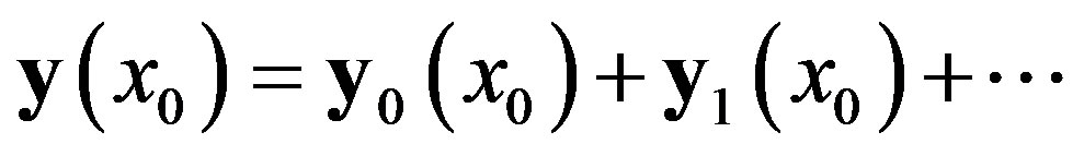
 , (2)
, (2)
where  is a correction to
 . The method of strained coordinates was first introduced by Lindstedt (1882) and other astronomers and now known as the Poincaré-Lighthill (PL) or Poincaré-Lighthill-Kuo method [4-8]. It is well-known that the PL method was designed originally for systems
 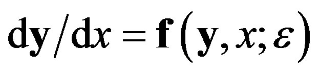 that depend critically on a small parameter
 , in order to render analytic series solutions uniformly convergent. However, we apply it here to problems like Equation (1) whose formulation is formally independent of a small parameter and for which standard coordinate perturbation methods are applicable. We use the adaptation in its renormalized form [9,10], which Dai [11] considers to be one of five important improvements in PL theory. Thus, we distinguish between standard and renormalized PL theory.
Section 2 shows the utility of the renormalized PL (rPL) theory in rendering variational equations homogeneous. Section 3 formulates the standard (std) fitting algorithm and Section 4 formulates its rPL generalization. Section 5 exemplifies the algorithm by means of a twopoint problem of stellar structure formulated in the Appendix, and compares the utility of each algorithm and the possibility of their combined usage. Section 6 discusses results.
2. Straining Coordinates
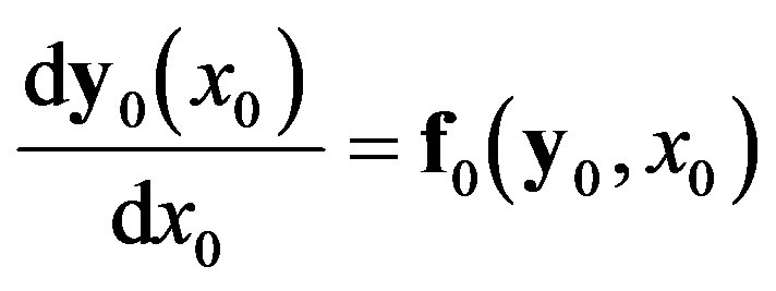
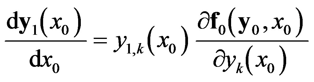
Apply Equation (2) to Equation (1) and separate orders to give to first order:
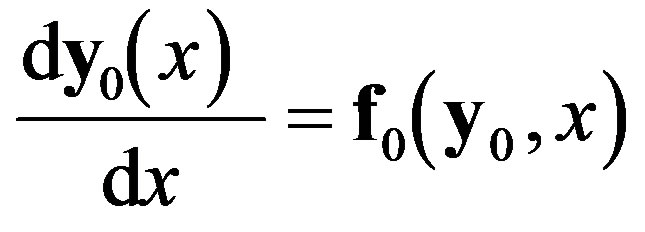 , (3)
, (3)
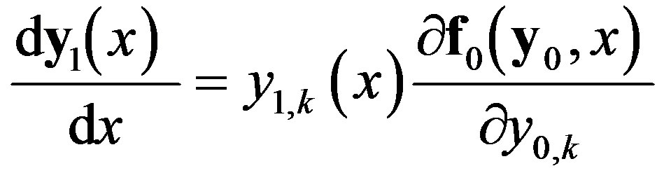 . (4)
. (4)
Following the standard PL procedure, x may be expanded as well as y(x), each as a function of a new independent variable :
:
 , (5)
, (5)
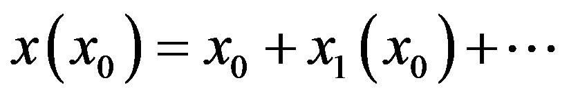 . (6)
. (6)
Function  stretches the independent coordinate x. Equations (5) and (6), when applied to Equation (1), give to zeroth and first order:
 , (7)
, (7)
 (8)
(8)
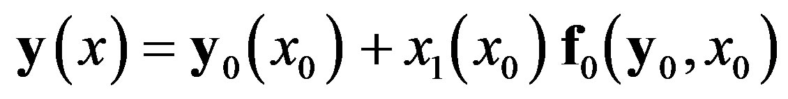
However, expansions (5) and (6) are not unique. Instead, apply Equation (6) to the equivalent standard expansion (2) [10], i.e. let:
 , (9)
, (9)
 , (10)
so that Equation (9) becomes:
 . (11)
On applying Equations (10) and (11) to Equation (1), and using the relation:
 , (12)
we discover that all terms in  cancel and:
 , (13)
 . (14)
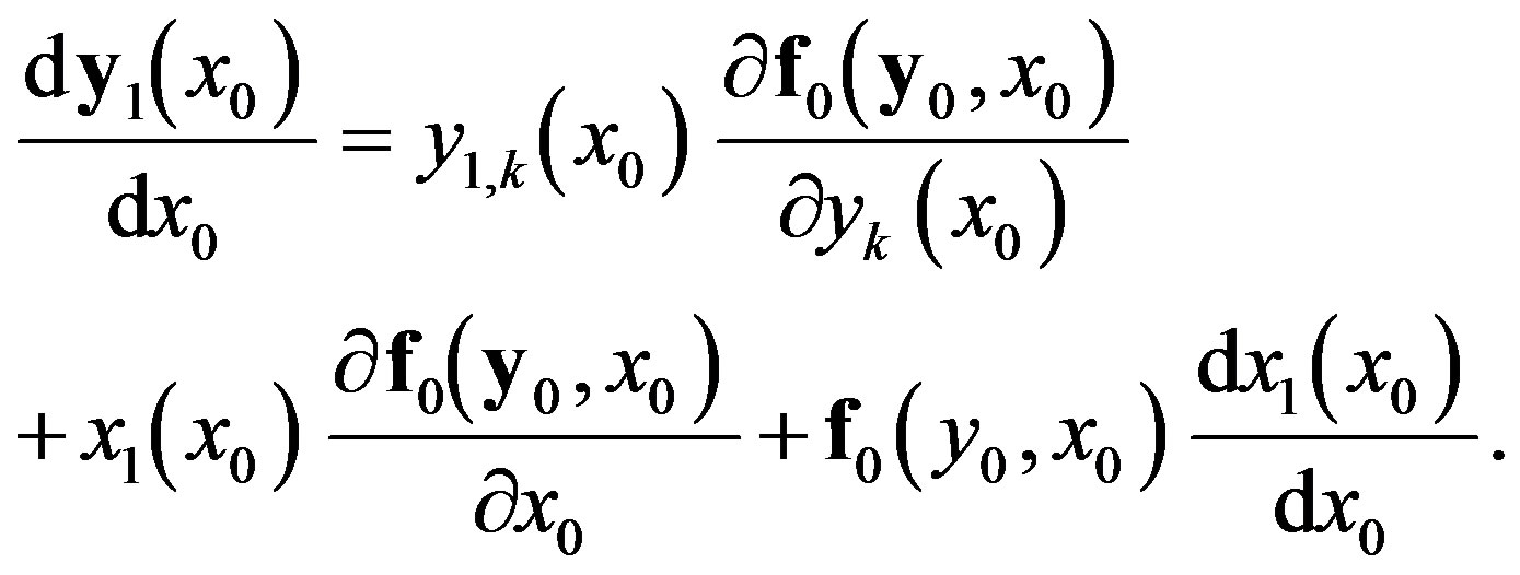
These are equivalent to Equations (3) and (4), except that the independent coordinate is x0 rather than x. The straining function  now appears only in expansions (10) and (11), and not in the differential Equation (8). On retaining terms to first order, these become the rPL perturbation expansions to first order:
 , (15)
 . (16)
Implementation of Equations (13) and (14), is straightforward as the conventional theory is recovered simply by setting , and x0 reverts to its original meaning x, as in Equations (3) and (4). In other words, in rPL, the straining feature may be applied after, and not during, the integration of the variational equations.
3. Standard Shoot and Fit
Frequently, in two-point boundary value problems, it is impossible to integrate from one boundary to the other without encountering some catastrophic result. This might occur while integrating toward a singular boundary, or when solutions become imaginary or unphysical. The standard (std) shoot and fit algorithm is designed to counter these difficulties, and in anticipation of its rPL generalization it is useful to spell it out.
Assume disjoint explicit boundary conditions, a normalized range, and for clarity distinguish integrations from each boundary by lower case and upper case variables. Throughout, let  and
and  For integrations from x = 0, Equation (13) is:
 , (17)
 , (18)
and from X = 1, it is:
 (19)
(19)
 , (20)
where  and
and  are trial values, and values
  and
and  may be transformed to zero. Suppose that trial integrations
  and
and  are wellbehaved up to a common point ξ. From Equations (17)- (20), generate J solutions
  for
for , and I solutions
  for
for , using initial conditions chosen as:
 (21)
(21)
 (22)
(22)
where , and
, and  are Kronecker deltas. Assume that the differences:
 , (23)
 , (24)
are linearly independent, where of course from Equations (17), (19), (21)-(24):
 , (25)
 . (26)
Linear superposition of Equations (23) and (24) gives:
 , (27)
 , (28)
where  are constants to be determined. Equations (2), (27) and (28) lead to:
 , (29)
 . (30)
Take the computed mismatches at ξ to be:
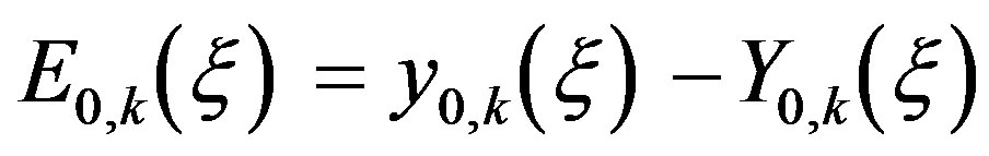 , (31)
which, from the difference of Equations (27) and (28) at ξ and the desired outcome , gives:
 . (32)
These are  linear algebraic equations in
  unknowns, whose solution gives
 , and Equations (29) and (30) give improved values:
 , (33)
 . (34)
4. The rPL Generalization
For , Equations (15) and (16) are:
 (35)
(35)
 , (36)
and for , they are:
 (37)
(37)
 . (38)
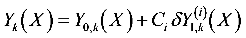
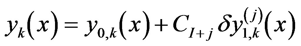
By Equations (7) and (13),  are numerically the same as
 . By Equation (15), analogues of Equations (29) and (30) are:
 (39)
(39)
 (40)
(40)
and the rPL version of Equation (32) is:
 (41)
(41)
4.1. Constraints
Functions  must satisfy two constraints: 1) In order that the independent variable be continuous at
 , a stretch
  must equal the compression
 , and vice versa; i.e.
 . (42)
2) With reference to Equations (39) and (40),  must be such as to nullify any singularities in
 .
.
4.2. Stretching
Functions  are otherwise arbitrary, but in the spirit of linearization let them vary linearly with their arguments. Equations (36) and (38) become:
 , (43)
 . (44)
Let the value in Equation (42) be:
 , (45)
where  is the amount of stretching/compression at the matching point. Thus:
 , (46)
 , (47)
and Equation (41) becomes:
 (48)
(48)
These are I + J equations in I + J + 1 unknowns, which require an extra equation for their solution.
4.3. Matching Condition
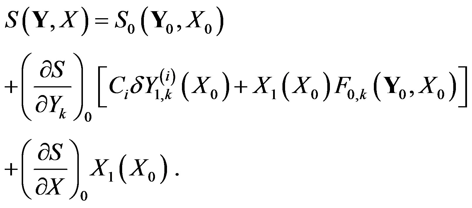
Let the (I + J + 1)th equation follow from matching s(y,x) and its functional twin S(Y,X) at the fitting point ξ. Expansions using Equations (39) and (40) are:
 (49)
(49)
 (50)
(50)
The desired outcome s(ξ) – S(ξ) = 0 and the computed difference:
 , (51)
lead to:
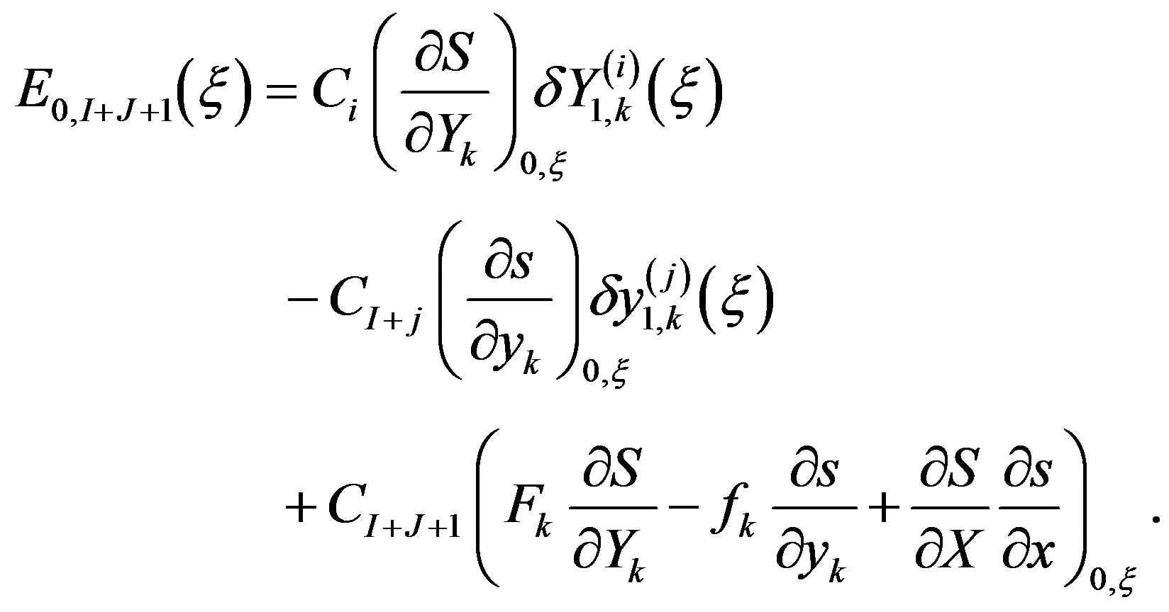 (52)
(52)
The I + J + 1 constants follow from the solution to Equations (48) and (52). With reference to Equations (39) and (40), improved guesses are:
 (53)
(53)
 . (54)
By Section 4.1, the last terms of Equations (53) and (54) must be finite or zero. If  nullify these terms, then the rPL Equations (53) and (54) resemble Equations (33) and (34) of std. In that case, the influence of stretching on the improved boundary conditions is nominally independent of
 , although of course stretching affects all
 ![]() through Equations (48) and (52).
through Equations (48) and (52).
4.4. Algorithm Option
For given trial values, relatively little extra computation time is involved in computing and solving the I + J + 1 algebraic Equations (48) and (52), compared to I + J Equations (32), whereupon the option exists to complete the next iteration using the rPL or the std algorithm. This requires devising a criterion by which to choose iterated values from one algorithm over values from the other.
From Equations (33) and (34), let the relative std corrections be:
 , (55)
 , (56)
From Equations (39) and (40), let the relative rPL corrections be:
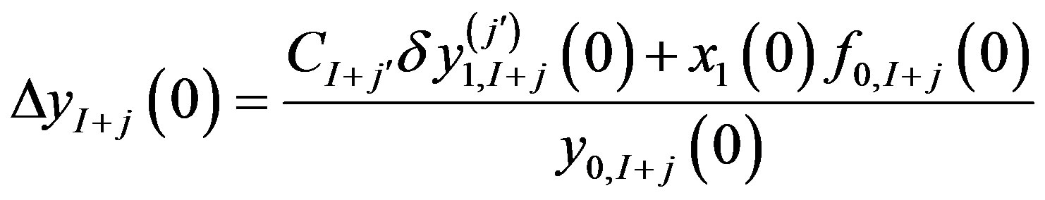 , (57)
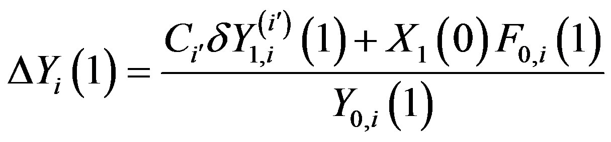 . (58)
As noted, quantities 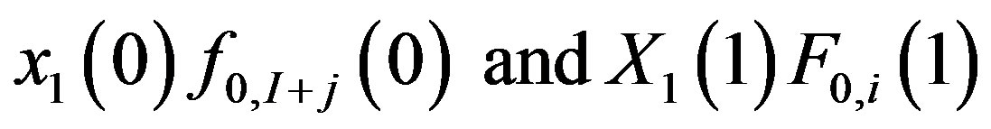 are proportional to the stretching constant
  and must be zero or finite. Define the sum of the squares of the relative corrections as:
 (59)
(59)
and let its value decide between the two options, i.e. between Equations (55) and (56), and Equations (57) and (58). Since relative errors obtain in Equation (59), it applies regardless of whether the converged solution is known (as it is in the present discussion), or not; i.e. Equation (59) is useful provided a way exists by which to decide between the available options. Section 5 contains empirical evidence concerning the better option. In practice, sequences of iterations generally have corrections derived from both algorithms; i.e. the two algorithms have the potential to widen the circle of convergence, since when one fails for any given iteration, the other may not. Thus, at the point of a failed iteration, an additional integration is the price to pay for the prospect of a wider circle of convergence.
5. An Illustrative Example
The shoot and fit method is applicable to an assortment of problems, including the two-point boundary problem of stellar structure [1,12]. Coordinate stretching has also proved useful in the study of rotating stars [13]. Stellar structure appears to be a suitable means for testing the rPL method against a known solution, for which it suffices to choose a relatively simple yet realistic model for a thirty-solar-mass (6 × 1031 kg) star. This is identical to early models [14,15], which were constructed less precisely and by different algorithms. The underlying physics is stated in the Appendix.
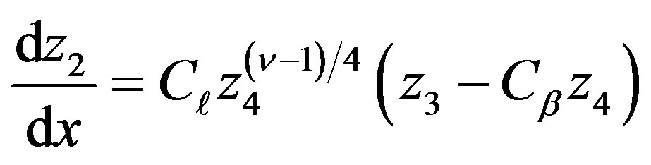
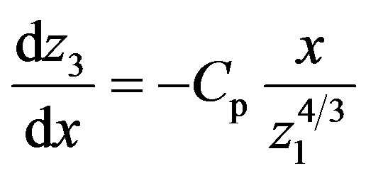
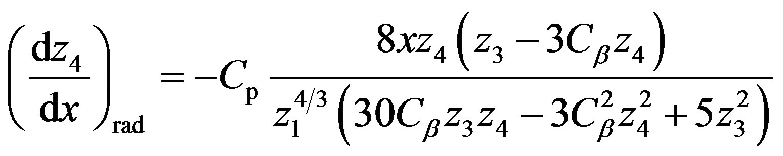
From transformations of Equations (76)-(81), (84), (85) of the Appendix, consider the problem:
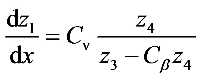 , (60)
 , (61)
 , (62)
 , (63)
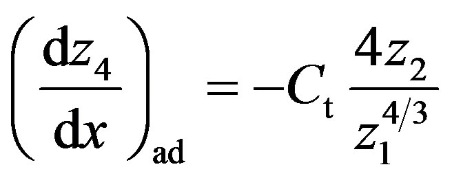 , (64)
where  is an index (see Appendix). Equation (63) or (64) obtains when
  is less or greater than
 , and positive dimensionless constants
  pertain to volume, luminosity, pressure and temperature (see Appendix). Boundary conditions are:
 . (65)
Physical arguments require . With foresight, and for present purposes, choose values
  that correspond to the converged solution in order that unknown boundary values converge to:
 . (66)
The unit boundary values of Equation (66) across the normalized range of the independent variable may be used here because the intent of Section 6 of this paper is to investigate the relative efficacy of algorithms by comparing trial values against the known solution. For the fourth-order system considered, the solution is characterized by four eigenvalues that correspond to four normalized ranges for the set . An auxiliary eigenvalue q marks the transition from one of Equations (63) and (64) to the other. Integration proceeds from each boundary to an arbitrarily chosen fitting point ξ, chosen throughout as 0.5. Integrations used the Odesolve (vector, x, b, npoints) routine of MATHCAD 14 [16], where vector is the array of sought solutions, x is the independent variable, b its terminal value, and npoints is the integer number of points used to interpolate the solution functions. Odesolve dynamically detects whether a system is stiff or not, and uses BDF (backward differentiation formula) or AB (Adams-Bashforth) methods respectively. Both methods use non-uniform step sizes, adding more integration steps in domains of greater variation. Subroutine root with tolerance TOL = 10−9 determined the location of the interface fraction q. The default precision is 17 significant figures.
Singular gradients at the boundaries require asymptotic developments, here limited to one significant term owing to the high precision of the calculations. Following Sections 3 and 4, lower and upper case variables distinguish integrations from x = 0 and x = 1. For small δx, δX, starting values are:
 , (67)
![]() , (68)
, (68)
 , (69)
 (70)
(70)
Figure 1 shows the normalized solution. Its derived boundary values and the auxiliary eigenvalue q agree to 1% or less with the aforementioned 30 solar mass model, with discrepancies explained by fitting by interpolation or by hand used previously.
Section 6.1 applies the std and rPL formulations. Integration proceeds through interfaces brought about by changes between Equations (63) and (64), and terminate at ξ = 0.5. To test the sensitivity of each independent variable to guesses in its unknown boundary value, we assign in turn the correct value 1 to all but one variable per Equation (65), to which we give values progressively farther from 1. Trial values are changed at intervals of ± 0.001 in the log, and convergence is considered continuous until the iteration fails to converge. Sometimes, convergence resumes for further changes in the guessed value, but it suffices for our purposes to apply the criterion of first failure uniformly across all cases. Execution ceases when one (or two) of the corrected guesses turns negative or when the number of iterations exceeds 20.
For the extra matching condition s(x), we require the continuity of a combination of variables unaccounted for by the original system. Consider the 6 products  and require:
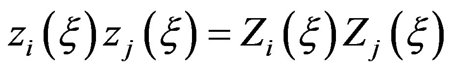 . (71)
None of these conditions is explicitly required in the problem formulation. Table 1 compares results for the 6 cases that use these rPL constraints simultaneously with the standard std algorithm. Iterations ceased upon satisfaction of the convergence criteria:
 , (72)
 , (73)
for i = 1,2 and j = 3,4. Results for entry 2 of Table 1 appear in Figures 2(a)-(d).
Devise two statistics by which to assess overall relative performance. For every , the extrema of the positive
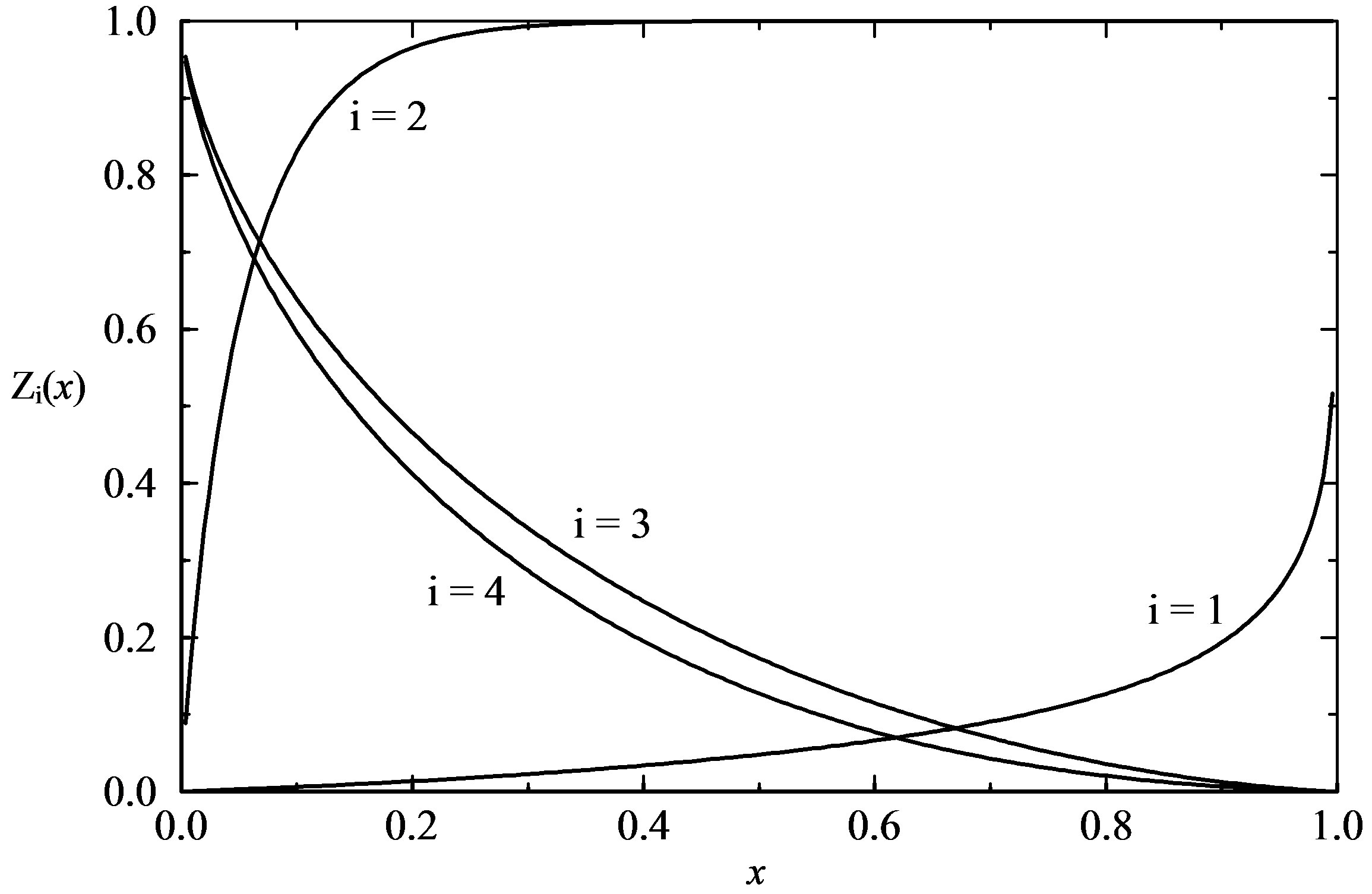
Figure 1. Solution to the posed problem. Subscripts identify volume (i = 1), luminosity (i = 2), total pressure (i = 3), radiation pressure (i = 4), and x is the normalized mass fraction.
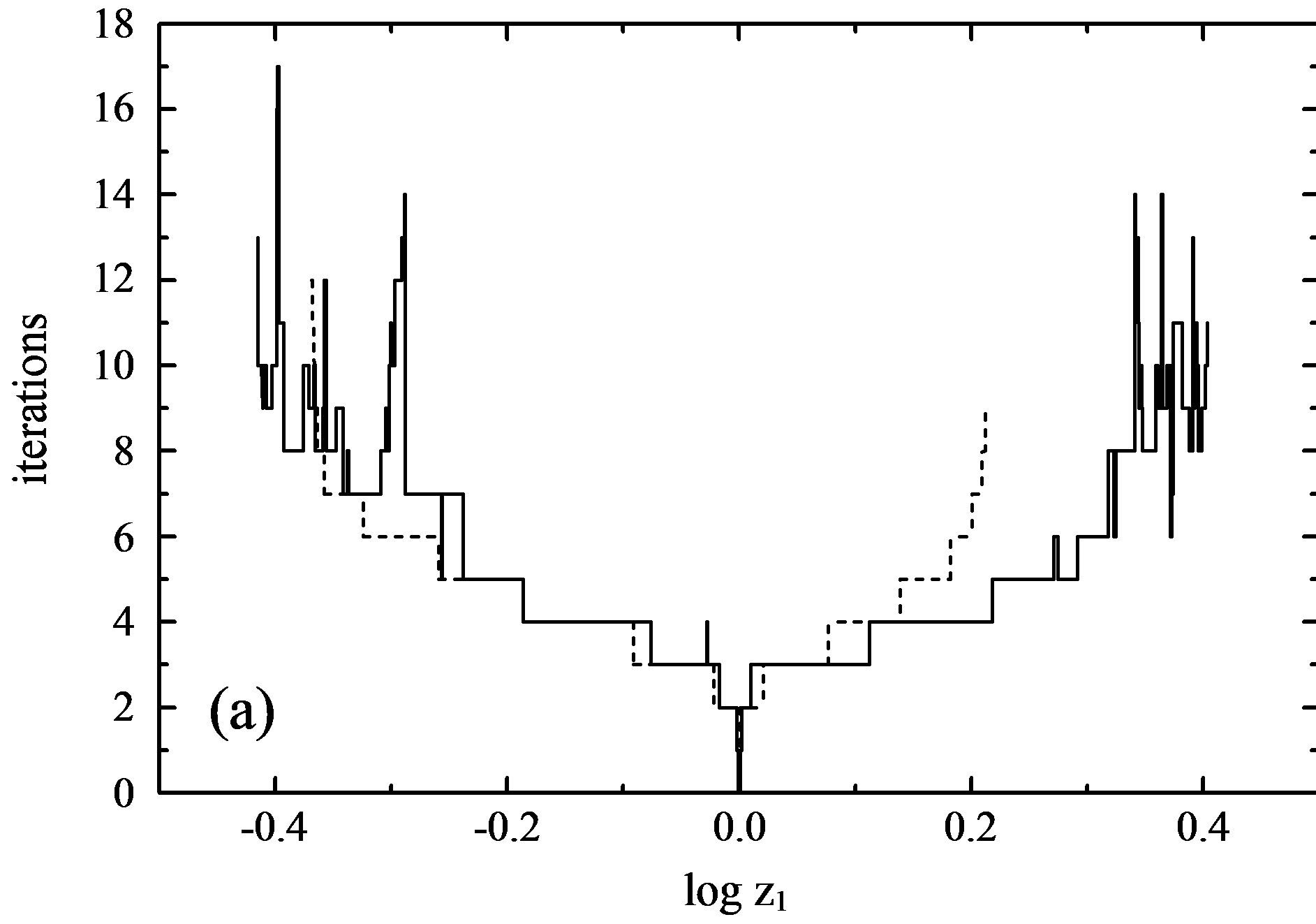
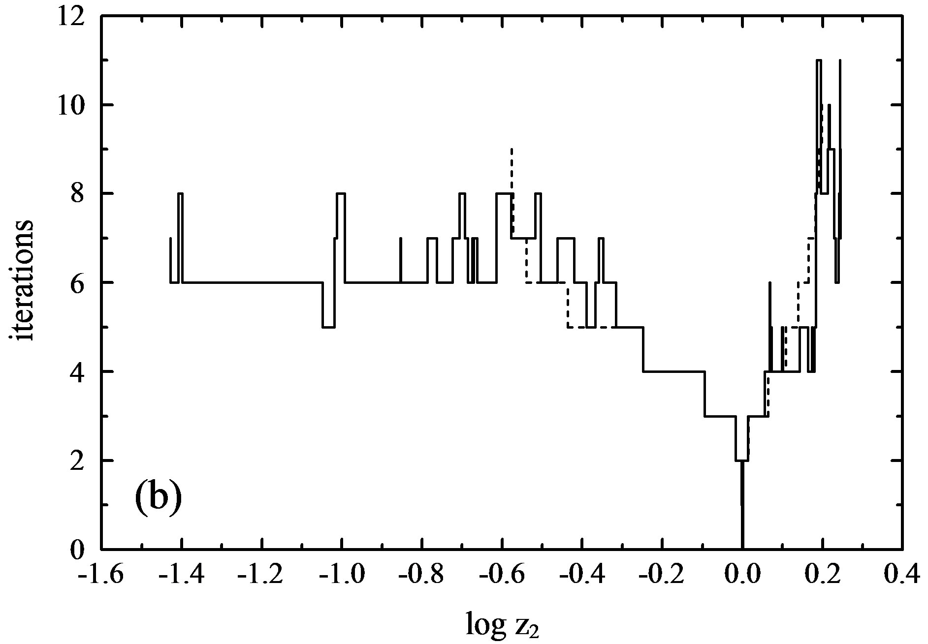
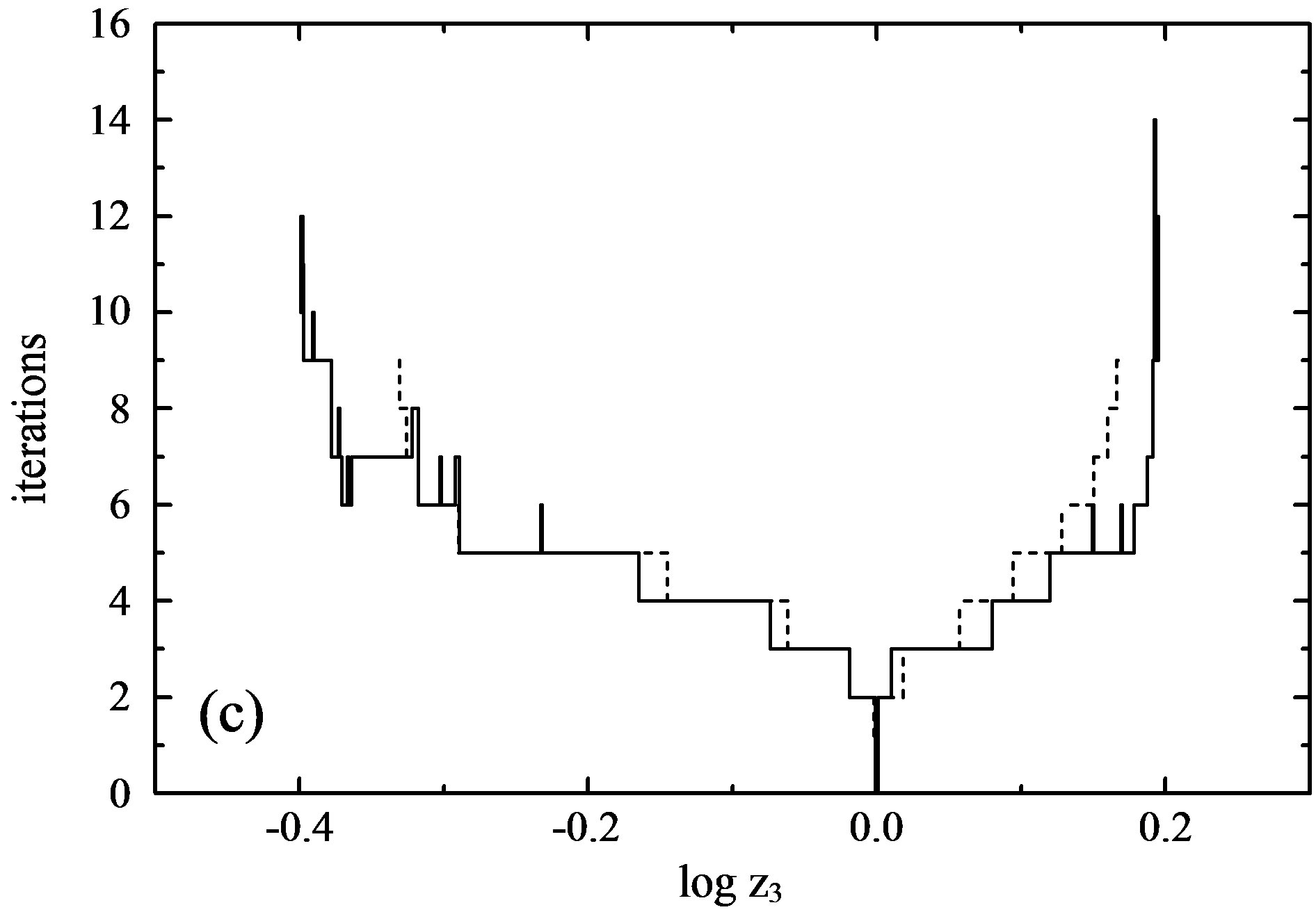
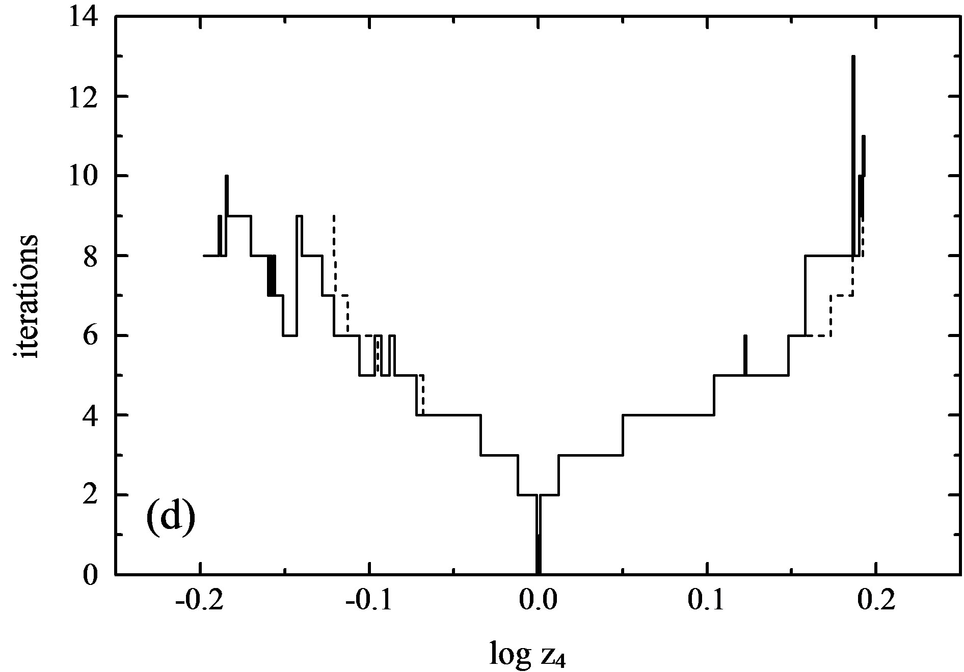
Figure 2. (a)-(d). Cases 1 and 2 of Table 1, showing the number of iterations to convergence by varying one unknown boundary value at a time, for the std algorithm alone (dashed line) and the std + rPL combined algorithm (solid line; see text).
and negative values of log are of interest, hence there is a total of
  for the four variables. Let ω be the number of cases for which
  is wider than that of the std algorithm, i.e. for which:
 . (74)
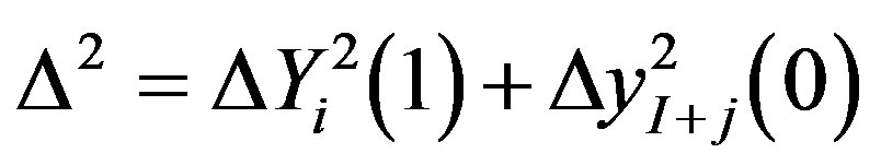
Choose the other statistic as the relative rms measure:
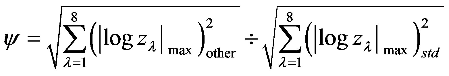 . (75)
6. Discussion
The std algorithm sets the standard by which to judge the efficacy of the rPL algorithm. It appears as Case 1 in Table 1, for which by definition ψ = 1. When the rPL algorithm alone is applied, only in about half the cases there is there an improvement over the std; i.e. for the present experiment, there is not much to choose between the two. Little is gained by showing these cases.
However, strength of the rPL lies in the similarity of Equations (4) and (14), which allows application of the rPL algorithm at little extra cost in computing time. We discover empirically (and counter-intuitively) that the better choice has the lesser value of Δ2 in Equation (59). This appears to minimize the tendency for iterations to diverge by over-correcting. Under these conditions, when the std option is tested simultaneously with the rPL (Cases 2-7 of Table 1), there is an improvement in convergence characteristics in all but one case. In Case 2, convergence occurs for as little as ≈3 × 10⁻² of the correct value. This phenomenon results from the fact that the model investigated is only a factor of 8 less than the Eddington luminosity limit at which stars are dynamically unstable (see Appendix), so that underestimates are computationally beneficial.
The excellent statistics of Case 2 in Table 1 attract attention. Figures 2(a)-(d) compare it to the std Case 1. Convergence in Case 2 is assisted by the extra rPL requirement of continuity in the product , where
  and
and  happen to be the two variables with the least uniformly-changing traces, as seen in Figure 1. For the present experiment, the comparative pathologies turn out to be virtual double-mirror images of one another and the product is quite well-behaved. It would seem a priori that these two variables would benefit most from an independent condition of continuity that involves them.
The chief result based on the problem definition and methodology here articulated, is that coordinate stretching
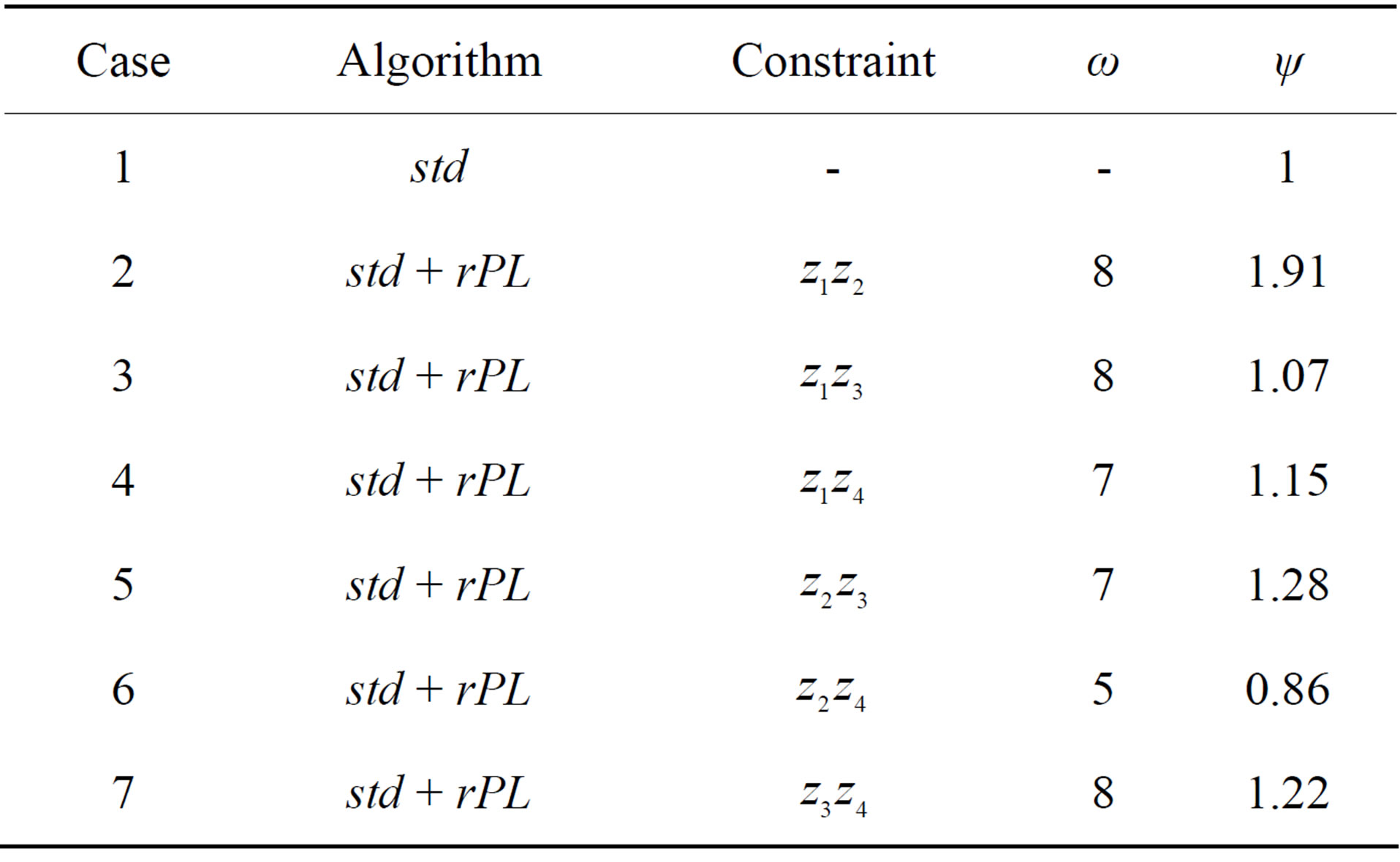
Table 1. Performance characteristics of the renormalized coordinate stretching (rPL) generalization of the standard (std) shooting and fitting algorithm, using the lesser value of Δ2 as the choice determinant (see text).
applied to numerical analysis may render dependent variables more uniformly convergent, if the extra condition is a simple function of variables with the least linear traces, provided this continuity condition is not otherwise part of the problem formulation. In a sense, this result for numerical analysis is analogous to the original intent of coordinate stretching, which is to render analytic series solutions uniformly convergent.
7. Acknowledgements
I thank Dr. Alan Stevens of the Institute for Mathematical Analysis and its applications for critiquing the programs used in this paper.
REFERENCES
- C. B. Haselgrove and F. Hoyle, “A Mathematical Discussion of the Problem of Stellar Evolution, with Reference to the Use of an Automatic Digital Computer,” Monthly Notices of the Royal Astronomical Society, Vol. 116, 1956, pp. 515-526.
- W. H., Press, S. A., Teukolsky, W. T. Vetterling and B. P. Flannery, “Numerical Recipes,” Cambridge University Press, Cambridge, 2007.
- S. M. Roberts and J. S. Shipman, “Two-Point Boundary Value Problems: Shooting Methods,” Elsevier, New York, 1972.
- A. Lindstedt, “Ueber Die Integration Einer Für Die Strö- rungstheorie Wichtigen Differentialgleichung,” Astronomische Nachrichten, Vol. 103, No. 14, 1882, pp. 211-220.
- H. Poincaré, “Les Méthodes Nouvelles de la Méchanique Céleste,” Gauthier-Villars, Paris, 1892.
- M. J. Lighthill, “A Technique for Rendering Approximate Solutions to Physical Problems Uniformly Convergent,” Philosophical Magazine, Vol. 40, 1949, pp. 1179-1201.
- A. S. Nayfeh, “Perturbation Methods,” Wiley, New York, 2000. doi:10.1002/9783527617609
- J. Kevorkian and J. D. Cole, “Perturbation Methods in Applied Mathematics,” Springer Verlag, New York, 2010.
- M. Pritulo, “On the Determination of Uniformly Accurate Solutions of Differential Equations by the Method of Perturbation of Coordinates,” Journal of Applied Mathematics and Mechanics, Vol. 26, No. 3, 1962, pp. 661-667. doi:10.1016/0021-8928(62)90034-5
- P. D. Usher, “Some New Algorithms for Stellar Structure,” Ph.D. Thesis, Harvard University, Harvard, 1966.
- S. Dai, “Poincaré-Lighthill-Kuo Method and Symbolic Computation,” Applied Mathematics and Mechanics, Vol. 22, No. 3, 2001, pp. 261-269. doi:10.1023/A:1015565502306
- J. Reiter, R. Bulirsch and J. Pfleiderer, “A Multiple Shooting Approach for the Numerical Treatment of Stellar Structure and Evolution,” Astronomische Nachrichten, Vol. 315, No. 3, 1994, pp. 205-234. doi:10.1002/asna.2103150304
- B. L. Smith, “Strained Coordinate Methods in Rotating Stars,” Astrophysics and Space Science, Vol. 47, No. 1, 1977, pp. 61-78.
- M. Schwarzschild and R. Härm, “Evolution of Very Massive Stars,” Astrophysical Journal, Vol. 128, 1958, pp. 348-360.
- R. Stothers, “Evolution of O Stars. I. Hydrogen-Burning,” Astrophysical Journal, Vol. 138, 1963, pp. 1074-1084.
- B. Maxfield, “Essential Mathcad,” Academic Press, Burlington, 2007.
Appendix
Consider a non-rotating, radially symmetric star of mass M = 6 × 1031 kg (30 solar masses) in quasi-hydrostatic equilibrium. Suppose that it is chemically homogeneous and that thermonuclear conversion of hydrogen to helium has just begun and is in a steady state. Assume that the material is entirely ionized and that it obeys the ideal gas law throughout. Let the relative mass abundances of hydrogen, helium and heavier elements be X = 0.70, Y = 0.27, and Z = 0.03, and let the mean molecular weight of the fully ionized gas in units of the proton mass H be
μ = .
.
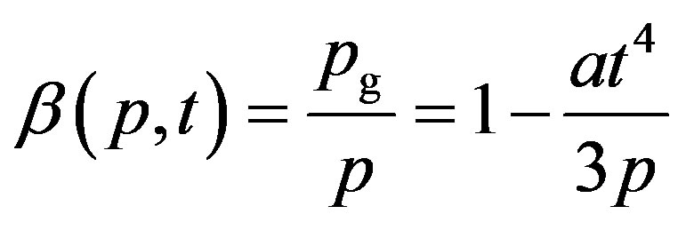
Constants are k (Boltzmann’s constant), c (the speed of light), a = 8π5k4/15c3h3 (the radiation density constant), h (Planck’s constant) and G (the gravitational constant). Variables are: v (volume), r (radius), ρ (material density), ℓ (luminosity or power), p total pressure, equal to the sum of radiation pressure 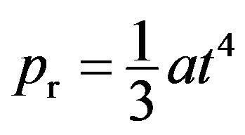 and gas pressure
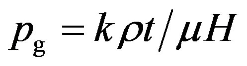 , where ρ is the material density, t temperature, and m mass fraction, i.e. the mass contained within volume v. In many applications, it is customary to choose m as the independent variable. Gradients are then:
 , (76)
 , (77)
 , (78)
 , (79)
 , (80)
where
 . (81)
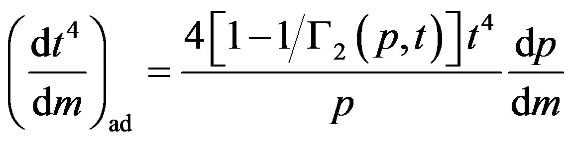
Equations (79) and (80) pertain to radiative and adiabatic convective energy transport for which the lesser of |dt/dm| applies. Physical conditions set limits 0 < β < 1. The ratio of gas specific heats at constant pressure and volume is , which is
  for an ideal gas. Γ2
is the second adiabatic exponent for a mixture of gas and radiation, for which
for an ideal monatomic gas and, in the present case, is limited to the range . Assume the opacity throughout is due to Thompson scattering by free electrons, κ = 0.02(1 + X) (kg–1·m2). Hydrogen fusion to helium is by the carbon-nitrogen-oxygen (CNO) cycle for which we let the combined C, N and O abundance be
 . Take the rate of energy generation to be
  Jkg–1·s–1, where ν = 15 and
  = 10–113.6Jm3·kg–2·s–1. Nomenclature in this formulation is standard, and symbols ε, k, X, Y, and Z are not to be confused with occurrences out of context.
During computation, starting values δx and δX were diminished until there were no further changes in the converged solution to a relative accuracy <10–6. For trial integrations sufficiently close to the true solution, we discover through trial and error or otherwise that radiative equilibrium obtains in the envelope and convective equilibrium in the core. Near the center  and Equations (76) and (77) give
 .
.
Near the surface , where it suffices to let p and t vanish. Equations (78) and (79) give:
 , (82)
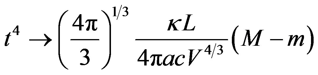 . (83)
Thus, boundary conditions are:
 . (84)
The stretching functions  in Equations (39) and (40) must be such as to cancel singularities at the boundaries. For the center, the terms of interest in Equation (35) both vary as
 , and condition 2 of Section 4.1 is met. For the surface,
  ,
,  ,
, . Both relevant products in
  of Equation (37) vary as
  and condition 2 of Section 4.1 is again met.
Define dimensionless variables:
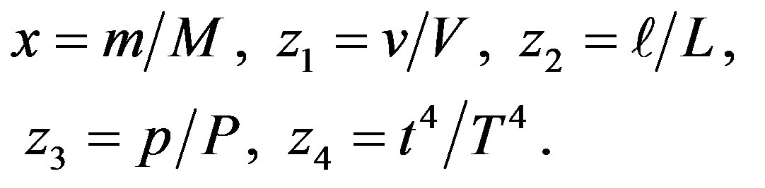 (85)
(85)
For present purposes, it is convenient to proceed with foreknowledge of the converged solution so that the unknown boundary values are normalized. The factors are ,
,  ,
,
 and
and . The transition between Equations (79) and (80) occurs at mass fraction
 . Dimensionless constants are:
 , (86)
 , (87)
 , (88)
 , (89)
 . (90)
Since , by Equations (81)-(83) in the limit
 ,
,  The quantity
  is the Eddington limit for the dynamical stability of a star whose opacity κ is constant, as it is in the present case, for which
 , which exceeds L by a factor of only 8.