American Journal of Plant Sciences
Vol.06 No.08(2015), Article ID:56719,21 pages
10.4236/ajps.2015.68128
Rhombic Analysis Extension of a Plant-Surface Water Interaction-Diffusion Model for Hexagonal Pattern Formation in an Arid Flat Environment
Bonni J. Kealy-Dichone1, David J. Wollkind2, Richard A. Cangelosi1
1Department of Mathematics, Gonzaga University, Spokane, USA
2Department of Mathematics, Washington State University, Pullman, USA
Email: dichone@gonzaga.edu
Copyright © 2015 by authors and Scientific Research Publishing Inc.
This work is licensed under the Creative Commons Attribution International License (CC BY).
http://creativecommons.org/licenses/by/4.0/


Received 26 March 2015; accepted 24 May 2015; published 27 May 2015
ABSTRACT
An existing weakly nonlinear diffusive instability hexagonal planform analysis for an interaction- diffusion plant-surface water model system in an arid flat environment [11] is extended by performing a rhombic planform analysis as well. In addition a threshold-dependent paradigm that differs from the usually employed implicit zero-threshold methodology is introduced to interpret stable rhombic patterns. The results of that analysis are synthesized with those of the existing hexagonal planform analysis. In particular these synthesized results can be represented by closed- form plots in the rate of precipitation versus the specific rate of plant density loss parameter space. From those plots, regions corresponding to bare ground and vegetative Turing patterns consisting of tiger bush (parallel stripes and labyrinthine mazes), pearled bush (hexagonal gaps and rhombic pseudo-gaps), and homogeneous distributions of vegetation, respectively, may be identified in this parameter space. Then that predicted sequence of stable states along a rainfall gradient is both compared with observational evidence and used to motivate an aridity classification scheme. Finally this system is shown to be isomorphic to the chemical reaction-diffusion Gray-Scott model and that isomorphism is employed to draw some conclusions about sideband instabilities as applied to vegetative patterning.
Keywords:
Tiger Bush, Pearled Bush, Nonlinear Stability, Threshold-Dependent Patterns

1. Introduction
In order to explain more fully the occurrence of tiger bush (or banded thicket) patterns in arid flat environments [1] , Kealy and Wollkind [2] introduced a two-component interaction-diffusion model system based on the Klausmeier [3] differential flow instability model but including the diffusion of surface water rather than its advection. That is, they considered the dimensionless coupled partial differential interaction-diffusion equation model for  plant biomass density and
  surface water content, where
  a two- dimensional spatial coordinate system and
  time,
time,
 (1.1)
(1.1)
 (1.2)
(1.2)
defined on an unbounded planar domain with
 . (1.3)
Here A and L are the rates of precipitation and evaporation for the water; R and M, the rates of water infiltration and biomass loss for the plants; J, the yield of plant biomass per unit water consumed; and  and
and , the constant dispersal and diffusion coefficients of the plants and water, respectively.
From a linear stability analysis of its possible critical points, Kealy and Wollkind [2] deduced that system (1.1)-(1.2) admitted both a bare ground trivial equilibrium point ( ,
, ) , which existed and was stable for all parameter values, and a homogeneous vegetation community equilibrium point
  which could generate a Turing [4] -type diffusive instability. They then performed a variety of weakly nonlinear instability analyses on that community equilibrium point finding from a one-dimensional analysis that it bifurcated supercritically to form a stationary striped vegetative pattern and from a two-dimensional hexagonal planform analysis that a close-packed array of vegetative gaps could occur in a narrow region flanking the marginal stability curve in their diffusive instability
  parameter space for the typical value of
  [5] . Finally, Kealy and Wollkind [2] identified these theoretical predictions with tiger and pearled bush patterns, respectively, and compared them with numerical simulations of Klausmeier’s [3] model system. Specifically, they showed that the predicted wavelength of the tiger bush patterns including the width ratio between stripes and interstripes was in very good quantitative agreement with the vegetative bands involving acacia trees in the Go-Gub area of Somaliland [6] . To make this comparison Kealy and Wollkind [2] employed the concept of low threshold patterns, originally introduced by Wollkind and Stephenson [7] and Boonkorkuea et al. [8] , without explicitly specifying the mechanism required to pose the proper threshold value for vegetative biomass associated with that methodology. After Cangelosi et al. [9] , who investigated a model for mussel bed patterning, in order to make this selection process more precise it is necessary for us to extend the weakly nonlinear stability analyses of Kealy and Wollkind [2] by performing a two-dimensional rhombic planform analysis of the community equilibrium point of (1.1)-(1.2) as well.
As a prelude to that investigation, we summarize the hexagonal planform results of Kealy and Wollkind [2] in Section 2. We perform the rhombic planform nonlinear diffusive instability analysis of the homogeneous vegetative equilibrium point of (1.1)-(1.2) in Section 3. In particular we find that, although square patterns of rhombic angle  are not stable, rhombic patterns of other characteristic angles do occur. In the process we introduce a threshold-dependent paradigm to interpret those stable rhombic patterns that differs from the implicit zero- threshold methodology usually employed for this purpose. We synthesize the results of Sections 2 and 3, in Section 4. These synthesized results can be represented by closed-form plots in
  parameter space for a fixed value of
 . From those plots, regions corresponding to bare ground and vegetative patterns consisting of tiger bush (parallel stripes and labyrinthine mazes), pearled bush (hexagonal gaps and rhombic pseudo-gaps), and homogeneous distributions of vegetation, respectively, may be identified in this parameter space. Then that predicted sequence of stable states along a rainfall gradient is both compared with observational evidence and used to motivate an aridity classification scheme based upon the vegetative patterning inherent to our system. Unlike strictly numerical procedures these analytical stability methods can be employed to determine quantitative relationships between system parameters and stable patterns which make it easier to compare theoretical predictions with field observations. Finally, we show our model to be isomorphic to the Gray-Scott chemical reaction- diffusion system and apply sideband instability results deduced for the latter to nonlinear vegetative pattern formation.
2. The One-Dimensional and Hexagonal-Planform Results of Kealy and Wollkind [2]
Kealy and Wollkind [2] found that the homogeneous vegetation equilibrium point of (1.1)-(1.2), which existed for , was linearly stable in the absence of diffusion when
 (2.1)
(2.1)
They performed a hexagonal planform analysis of that community equilibrium point of system (1.1)-(1.2) by seeking a solution to it that to lowest order satisfied
 (2.2)
(2.2)
where, for  even permutations of (1, 2, 3),
 (2.3)
(2.3)
 (2.4)
(2.4)
with an analogous expansion for .
.
Their one-dimensional pattern formation results can be deduced by taking
 (2.5)
(2.5)
in (2.2) and (2.3)-(2.4). From a linear stability analysis Kealy and Wollkind [2] found that the components of the maximum point of the marginal curve in their wave number squared-bifurcation parameter two-dimensional space were given by
 (2.6)
(2.6)
where
 (2.7)
(2.7)
with  being the most dangerous mode of linear theory. Then, for fixed
  and
and ,
,  when
when ,
,  when
when , and
, and  when
when . Thus the locus
  served as a marginal stability surface in
  three-dimensional space. In addition the locus
  where
where
 (2.8)
(2.8)
depicted in Figure 1, served as a similar surface in  space.
Under the conditions of (2.5), the amplitude-phase equations of (2.3)-(2.4) reduced to the Landau equation
 (2.9)
(2.9)
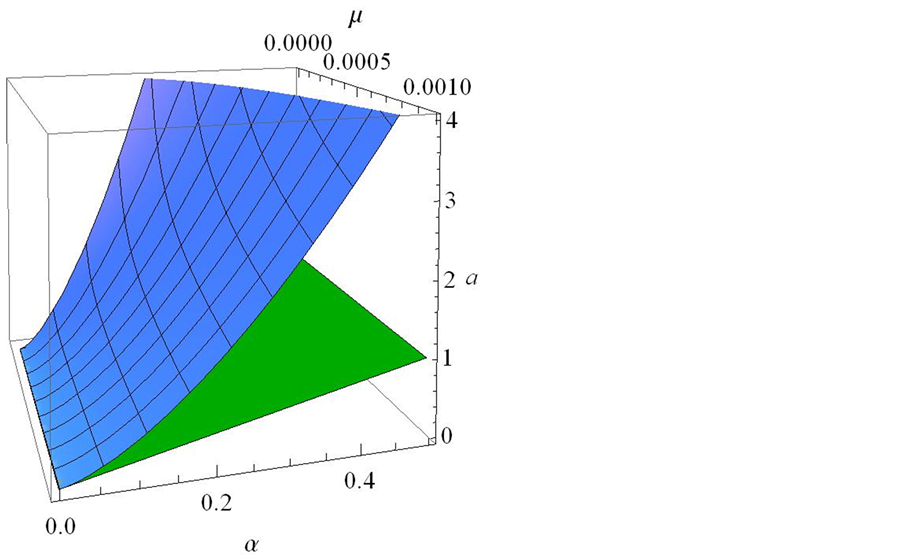
Figure 1. Three-dimensional plots of the marginal stability surface  of with
  and the planar surface
  for
for  and
and .
.
From their one-dimensional nonlinear stability analysis Kealy and Wollkind [2] found that
 (2.10)
where  is plotted versus
  in Figure 2 for
  and
and . That Landau constant, given explicitly in the Appendix, had the asymptotic representation [2]
 (2.11)
where
 (2.12)
Figure 2 consists of two parts: A left-hand part for which  has been plotted for the same
  -domain as in Figure 1, namely
 ; and a right-hand one, which is an enlargement of the former restricted to the lower end of that
  -domain. From Figure 2, it can be observed that this curve has a zero at
  characterized by
 (2.13)
where
 (2.14)
and a linear asymptote of the form  which is almost coincident with it when the
  -scale of Figure 1 is employed. Since for ecologically relevant values of
 ―e.g.,
  and
and  [3] , the constraint
  was satisfied identically should
  [5] , Kealy and Wollkind [2] considered
  positive and concluded that when
 , the community equilibrium point was stable giving rise to a uniform homogeneous vegetative distribution while when
  a re-equilibrated state of stationary
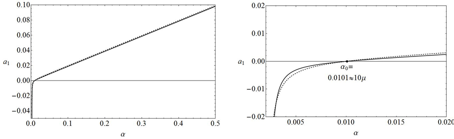
Figure 2. Plots of the Landau constant  of versus
  for
for  with
with  (solid line) and its asymptotic approximation as
  given by (2.11) (dashed line). The right-hand panel is an enlargement to illustrate the behavior of the approximation near
 .
.
parallel vegetative stripes resulted with amplitude  and dimensional and dimensionless wavelength
 (2.15)
respectively.
The one-dimensional pattern formation results of Kealy and Wollkind [2] are summarized in the  plane of Figure 3 for
 The traces of the Turing bifurcation boundary surface
  and the plane
  of Figure 1 are plotted in that figure versus
  when
when . Then the regions
 ,
,  and
and  can be identified with bare ground, stationary striped vegetative patterns, and homogeneous vegetative distributions, respectively, in that parameter space. Finally note that
  and
and  should
  while (2.1) is satisfied identically for
 .
.
Wishing to refine their one-dimensional pattern formation predictions summarized in Figure 3, Kealy and Wollkind [2] next considered the full two-dimensional hexagonal planform expansions of (2.2) and (2.3)-(2.4). Since  and
and  were given by their one-dimensional analysis only
  and
and  needed to be evaluated. Proceeding in the same manner as they did with the one-dimensional expansion to determine
 , Kealy and Wollkind [2] employed the relevant Fredholm-type solvability conditions to yield explicit formulae (see the Appendix) for the remaining two Landau constants
 (2.16)
catalogued the critical points of equations (2.3)-(2.4); summarized their orbital stability behavior; and identified the potentially stable ones with various vegetative patterns obtaining the following critical point identifications: I, homogeneous distributions; II, stripes , spots; and
 gaps. Note, in this context, that I and II represent the same identifications as catalogued in Figure 3. The contour plots relevant to critical points
  are depicted in Figure 4, where Figure 4(a) is for
  and Figure 4(b), for
 . Here, the spatial variables are measured in units of
  while dark and light regions correspond to high and low densities, respectively, in accordance with the aerial photographs appearing in [6] and [10] .
Kealy and Wollkind [2] first determined that critical point I was stable provided . Then, since the existence and stability of critical points II and
  depended upon them, they examined the signs of
 ,
,  ,
,  , and
, and  as functions of
  by plotting those quantities as well as
  versus
  for
for  with
with  which we reproduce in Figure 5 for
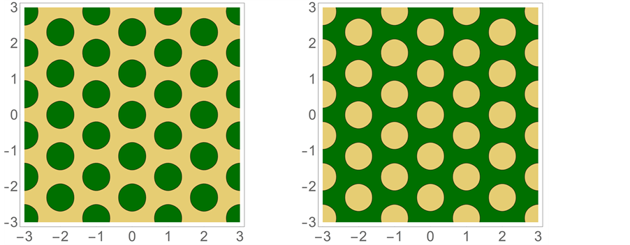
 . Kealy and Wollkind [2] found that
  was identically positive while all the other relevant quantities in Figure 5 were positive for
 , having zeroes less than
 . Thus, since
  only critical points II and
  could be stable [11] . Note, in this context, that critical point
  cannot be stable under these conditions and hence this model may only predict vegetative gaps but not spots. Finally, Kealy and Wollkind [2] represented their stability results graphically in the
  plane by generating the loci associated with
  with
with , 1, and 2,
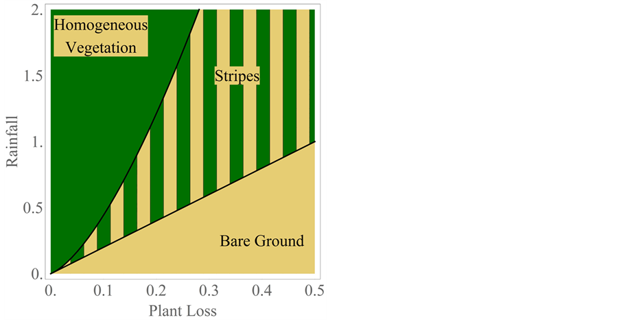
Figure 3. Stability diagram in the  plane for our one- dimensional interaction-diffusion model system with
 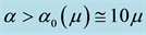 and
and , denoting the predicted vegetative patterns. The curves depicted in this figure are cross-sections of the plane
  with the surfaces of Figure 1. Hence, the upper one is the Turing boundary
  with
with  and the lower one, the straight line
 .
.
 (a) (b)
Figure 4. (a) A contour plot of the hexagonal array of spots for ; (b) A contour plot of the hexagonal array of gaps for
 .
.
respectively, for
 (2.17)
from (2.8)
Figure 5. Plots of ,
,  ,
,  , and
, and  of (A.1) and (A.2) versus
  for
for  with
with , where plots of
  and
and  are presented for purposes of comparison.
 (2.18)
where
 (2.19)
We plot these loci along with those of Figure 3 in Figure 6 for  and
and . Using the stability criteria for critical points II and
  [11] , Kealy and Wollkind [2] made the morphological predictions that stripes could occur for
  while hexagonal close-packed arrays of vegetative gaps could occur for
 . Since homogeneous distributions of vegetation could occur for
 , there were two regions of bistability: Namely,
  , where homogeneous distributions and gaps could occur; and,
  , where gaps and stripes could occur. Further bare ground occurred for
 .
.
We close this section with the observation that in order to retain only terms through third-order in our expansions of (2.3)-(2.4) its Landau constants must be in the relation [12]
 (2.20)
which is satisfied for those quantities as depicted in Figure 5.
3. Two-Dimensional Analysis: Rhombic-Planform Nonlinear Stability Results
Wishing to refine further the two-dimensional hexagonal planform predictions summarized in Figure 6 and to investigate more precisely the possibility of occurrence of the low-threshold tiger bush patterns observed by Levefer and Lejeune [6] , we next consider a rhombic-planform solution of system (1.1)-(1.2) of the form [7]
 (3.1)
(3.1)
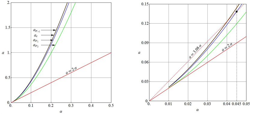
Figure 6. Plots of ,
,  , and
, and  of (2.19) as well as
  and
and  of Figure 3 versus
  for
for  with
with . The right-hand panel is an enlargement depicting the intersection point between the vertical line
  and the
  locus
locus  (see Section 4). Note that the plots of
  and
and  virtually coincide.
where
 (3.2)
(3.2)
with an analogous expansion for , such that
 (3.3)
(3.3)
 (3.4)
(3.4)
Here we are employing the notation  for the coefficient of each term in (3.1) of the form
 The terms on the right-hand side of (3.3)-(3.4) can be deduced by examining the amplitude functions in (3.1) proportional to
  and
and , respectively. Then substituting this rhombic-planform solution of (3.1)-(3.2) into system (1.1)-(1.2), we obtain a sequence of problems, each of which corresponds to one of these terms. In order to catalogue the solutions of those problems we introduce the following notation. Denoting the interaction terms in (1.1)-(1.2) by
 (3.5)
(3.5)
we define the expansion coefficients
 (3.6)
(3.6)
which are tabulated below:
 (3.7)
(3.7)
Solving those problems we find that
 (3.8)
(3.8)
while applying the same method of analysis, as employed for deducing (A.1) and (A.2), to the ,
,  ,
,  system yields the Fredholm-type solvability condition for the second rhombic-planform third-order Landau constant
 (3.9)
(3.9)
where the components of
 (3.10)
as well as the solutions for the relevant second-order systems are catalogued in the Appendix.
Having developed these formulae for its growth rate and Landau constants, we now turn our attention to the rhombic-planform amplitude Equations (3.3)-(3.4), which possess the following equivalence classes of critical points :
:
 (3.11)
Assuming that  and investigating the stability of these critical points one finds that [7] :
 (3.12)
Note that I and II, as in the one-dimensional analysis of the previous section, represent the uniform homogeneous and supercritical banded states, respectively, while V can be identified with a rhombic pattern possessing characteristic angle  [7].
[7].
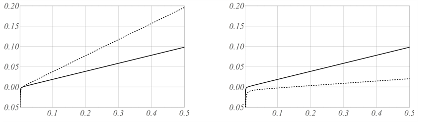
We now use these criteria to pursue those goals stated at the beginning of this section. Toward that end, we first plot  versus
  for
for ,
,  ,
,  , and
, and  with
with  in the four parts of Figure 7, respectively, each of which also includes a plot of the
  of Figure 5. Here
  represents a limiting case where the rhombic pattern reduces to parallel stripes while
  represents a square planform (see below). Upon comparing
  with
with  in Figure 7, we see that
  for
for ,
,
 (a) (b)
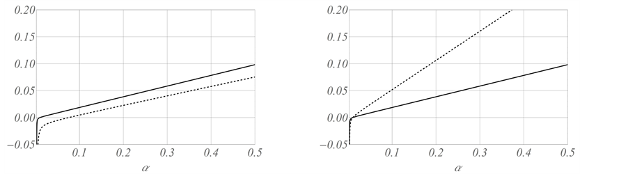 (c) (d)
Figure 7. Plots of  of (3.9)-(3.10) (dashed curve) and
  of (solid curve) versus
  with
with  for
for  (a) 0; (b)
 ; (c)
; (c) , and (d)
 .
.
 for
for  and
and  and
and  for
for . Hence, since the latter condition violates the stability criterion of (3.12), we can conclude that stable square patterns do not occur for this problem when
 . From (3.11)-(3.12) we can deduce that, to demonstrate conclusively a rhombic pattern of angle
  exists and is stable, we must show that
  or, equivalently after Geddes et al. [13] defining the ratio of these Landau constants by
 , that
 (3.13)
provided, in addition, that  or
or . Next, we plot this ratio of Landau constants
  versus
  for the fixed values of
  and
and  in Figure 8. Restricting ourselves to the interval of interest
 , we see from this figure that there are two bands of stable rhombic patterns flanking
  for
for  or
or  when
when  where
where
 (3.14)
which have been designated by vertical lines. Both of these lie between  and
and , which have been designated by horizontal lines. In particular, consistent with Figure 7(b) and Figure 7(c) when
 , note that
  while
while . In this context, observe that, for the special case of
 , (3.13) reduces to
  or
or . Observe from Figure 8 that
 (3.15)
which is consistent with Figure 7(a). Also note that this figure has been drawn for the extended interval  in order to demonstrate graphically the symmetry about
  characteristic of rhombic patterns since
 (3.16)
Here, properties (3.15) and (3.16) are a consequence of mode interference occurring exactly at  and modal interchange, respectively [14] .
We have deferred until now a detailed morphological interpretation of the rhombic patterns that can be identified with critical point V for the values of the characteristic angle  relevant to Figure 7. Then, to lowest order, the equilibrium vegetative pattern associated with that critical point satisfies
 (3.17)
where
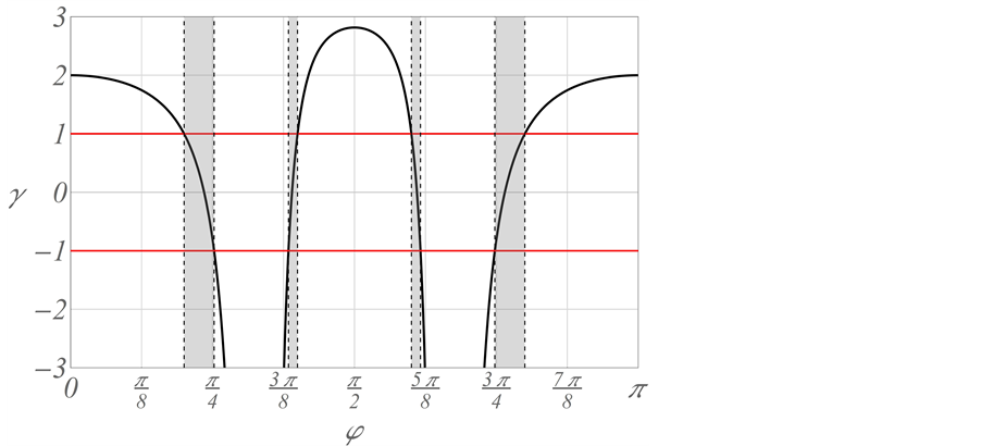
Figure 8. A plot of  of (3.13) versus
  for
for  and
and .
.
 (3.18)
The three parts of Figures 9-12 are threshold contour plots of (3.18) for ,
,  ,
,  , and
, and  with threshold values of
 , 0, and 1, respectively. Here the spatial variables are again being measured in units of
  and regions exceeding that threshold in each part appear dark while those below it appear light. Hence from left to right the parts of these figures correspond to what Wollkind and Stephenson [7] , Boonkorkuea et al. [8] , and Cangelosi et al. [9] termed lower, zero, and upper threshold patterns, respectively. In this context note that
 . Traditionally, most pattern formation analyses of this type have used the dimensional homogeneous vegetative solution value of
  where [2]
 (3.19)
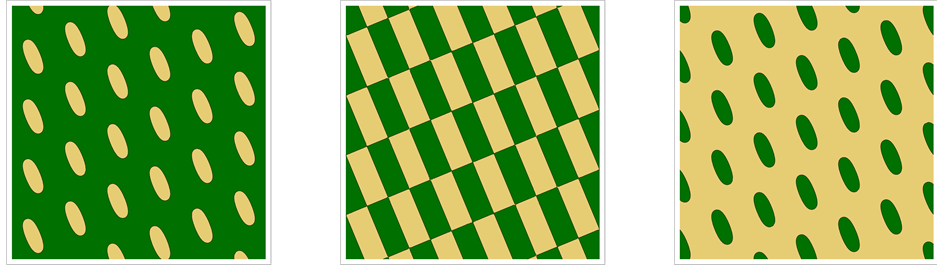
Figure 9. Striped patterns relevant to  of (3.17)-(3.18) for
  with threshold values from left to right of (a)
 , (b) 0, and (c) 1.
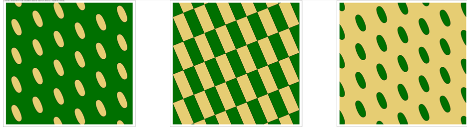
Figure 10. Rhombic patterns relevant to  of (3.17)-(3.18) for
  with threshold values from left to right of (a)
 , (b) 0, and (c) 1.
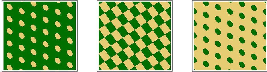
Figure 11. Rhombic patterns relevant to  of (3.17)-(3.18) for
  with threshold values from left to right of (a)
 , (b) 0, and (c) 1.
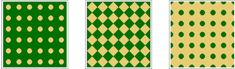
Figure 12. Square patterns relevant to  of (3.17)-(3.18) for
  with threshold values from left to right of (a)
 , (b) 0, and (c) 1.
as the threshold to trigger the color change from light to dark (see Figure 4). Thus all spatial regions characterized by  appear light and those characterized by
 , dark, where again light regions correspond to low plant biomass density or bare ground and dark ones to high plant biomass density. This is equivalent to our zero threshold cases of Figures 9-12 upon assuming, without loss of generality, that
 Explicitly denoting
 (3.20)
Kealy and Wollkind [2] plotted  for
for , 0, and 1, as well as the marginal stability curve
  in the
  plane with
  for
for . Analogous to the morphological stability predictions of Figure 6, they concluded that homogeneous distributions could occur for
 , stripes for
 , and gaps for
 . We reproduce these results in Figure 13 for
  and defining
 (3.21)
adopt the protocol that  represents this threshold instead. Then, where
  or
or , the lower threshold patterns of Figures 9-12 would occur while, where
  or
or , the upper threshold patterns would occur. Given their similarity of appearance to the hexagonal vegetative patterns of Figure 4 we shall now label these lower and upper threshold rhombic vegetative arrays as pseudo gaps and pseudo spots and denote them by
  and
and , respectively. In this context, after Sekimura et al. [15] , the lower and upper threshold patterns of Figure 12 could be labeled as square gaps and square spots, respectively.
4. Synthesis, Aridity Classification Scheme, and Comparisons
We first wish to synthesize the morphological stability predictions summarized in Section 2 and developed in Section 3, respectively. To do so, we begin by considering our rhombic pattern formation results of the latter section in conjunction with the hexagonal pattern formation ones of the former section. Extrapolating from the conclusions of Golovin et al. [16] and Schatz et al. [17] , who demonstrated theoretically and experimentally, respectively, that square patterns only occurred for Marangoni convection with poorly conducting boundaries in the neighborhood of the marginal stability curve where supercritical Bénard cells but not rolls would normally be predicted from a hexagonal planform analysis, we can deduce that our stable rhombic vegetative patterns will only occur in the region of parameter space satisfying  in Figure 13 or, equivalently,
  in Figure 6. Since
  (see Figure 13), these stable rhombic patterns will be of the lower threshold
  variety or pseudo gaps. Hence, we can synthesize our morphological stability predictions of Section 2 and Section 3 by means of Table 1 which identifies the relevant regions of parameter space in Figure 6 and Figure 13 with the stable vegetative patterns that can occur in those regions.
Observe from Figure 6 that the plot of  seems to be visibly coincident with the Turing boundary
 . In this context, note that, for the parameter value of
  relevant to tiger bush [3] ,
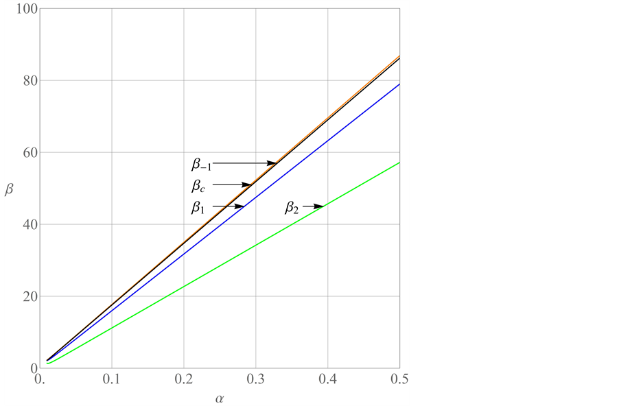
Figure 13. Plots of the marginal curves of (2.6)-(2.7) and (3.20)-(3.21) versus  with
with .
.
 (4.1)
(4.1)
The locus  is designated by the vertical line appearing in Figure 6. Since the behavior portrayed in (4.1) occurs for all
  and deviations of this sort are well within the allowable observational error, we shall take
 (4.2)
(4.2)
in what follows. Under this simplification the rainfall column of the morphological stability predictions of Table 1 reduces to that of Table 2.
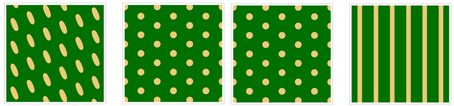
We represent generic versions of these patterns in Figure 14. Here we have made use of the fact that  serves as the critical threshold which can be deduced from our adoption of
  for that purpose in conjunction with Table 1. Hence we may conclude that lower, zero, or upper threshold patterns occur for a greater than, equal to, or lesser than
 , respectively. Note that the gap and pseudo gap patterns depicted in Figure 14 are of the lower threshold type since they occur for
  as opposed to the gap pattern of Figure 4(b) which was implicitly of the zero-threshold type while the depicted stripe patterns are of all the three threshold types appearing in Figure 9. We now after von Hardenberg et al. [18] offer an aridity classification scheme along a rainfall gradient in Table 3 based upon the results of Table 2 particularized to those values of (4.1) for
 and
and .
.
Kealy and Wollkind [2] compared their theoretical predictions with relevant observational evidence involving periodic self-organized vegetative patterns of tiger and pearled bush occurring in homogeneous ecosystems (reviewed by Rietkerk et al. [19] ). Tiger bush tends to consist of parallel vegetative stripes. When the ground surface slopes, these stripes migrate upslope while when that surface is practically flat static banded vegetation patterns result. Couteron et al. [1] catalogued those differences between these two-types of banded thicket patterns. The static banded states provided good qualitative agreement with tiger bush patterns found in arid flat environments while the upslope migrating stripes predicted by Klausmeier [3] , Sherratt [20] , and Sherratt and Lord [21] provided such agreement with those found in sloping environments. Hence, Wollkind and Kealy [2]
 (a) (b)
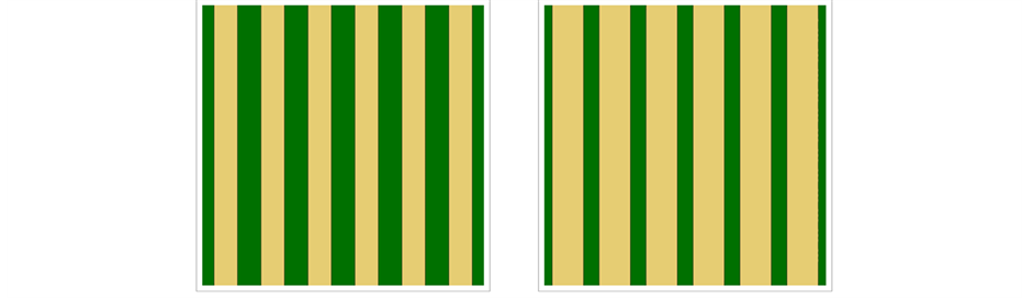 (c) (d)
Figure 14. Predicted generic vegetative patterns relevant to Table 3 for (a)  Pseudo Gaps and Gaps; (b)
  Gaps and Low-threshold Stripes; (c)
 , Zero-threshold Stripes; (d)
 , High-threshold Stripes.

Table 1. Synthesized morphological stability predicitions for Figure 6 and Figure 13.
Table 2. Simplified morphological stability predictions along a rainfall gradient.
identified their parallel stationary diffusive instability stripes with those tiger bush patterns found on plateaus. In order to demonstrate that their model also provided good quantitative agreement with observed tiger bush patterning, they considered Figure 1 of Lefever and Lejeune [6] which is a photograph of regular parallel stripes
Table 3. Aridity classification scheme along a rainfall gradient for .
.
consisting of Acacia bussei trees in the Go-Gub area of Somaliland. These stripes are about 100 m wide while the width of the separating interstripes is about 50m. Thus the dimensional wavelength associated with this pattern is approximately
 (4.3)
(4.3)
To compare these predicted pattern wavelengths of (2.15) with this result, they first reformulated the wavenumber expression of (2.6) by solving the marginal stability curve  for
for  to obtain
 (4.4)
(4.4)
and then substituting (4.4) into (2.6) found that
 (4.5)
(4.5)
Now, employing this formula of (4.5) in (2.15) and making use of the definition of  from (1.3), they represented
 (4.6)
(4.6)
and
 (4.7)
(4.7)
Introducing the evaporation rate and surface water diffusion values from Klausmeier [3] and Rietkerk et al. [5] , respectively,
 (4.8)
(4.8)
into (4.6)-(4.7) then yielded
 (4.9)
(4.9)
which, upon comparison with (4.3), implied that
 (4.10)
Finally, inverting (4.6), Kealy and Wollkind [2] obtained
 (4.11)
where
 (4.12)
They then used (4.11)-(4.12) to plot lines of various constant wavelength  in the striped patterned region in their figure analogous to our Figure 3 which we reproduce in Figure 15 but for
  with
with . From (4.11)-(4.12), Kealy and Wollkind [2] deduced that the
  contour in Figure 15 satisfied the linear relationship
 (4.13)
Recalling that , this corresponds to
  and is consistent with Klausmeier’s [3]
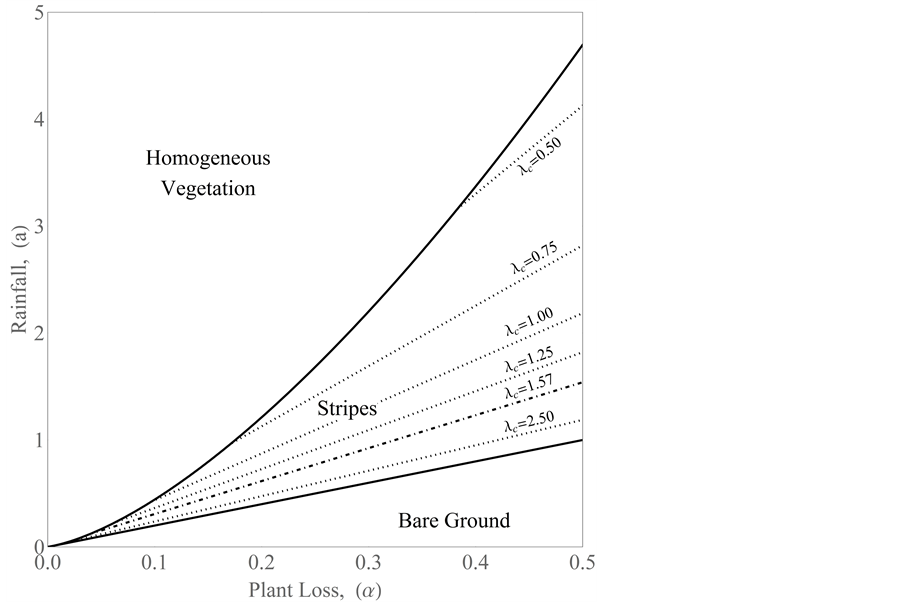
Figure 15. A reproduction of the  plane of Figure 3 denoting the lines of various constant wavelength
  as determined by (4.11)-(4.12) in the striped vegetation patterned region. Here the line
  corresponds to
 .
.
assertion that . These results are catalogued in Table 4 and represented graphically in Figure 6 by the point of intersection between the vertical line
  and the linear locus of (4.13).
Observed from Table 2 and Figure 14, that stripes of this sort, occurring at the upper bound of allowable  - values for such patterns in what we have classified as the semiarid region by Figure 3, are of the lower-threshold variety. In order to obtain the required 2 to 1 width ratio between stripes and interstripes, it is only necessary that we adopt a critical threshold of
  [2] . Note that this corresponds to the lower threshold part of Figure 9 which was for a threshold value of
  since
since  when
when . Anticipating this result, that part of Figure 9 has been employed as the representative lower-threshold stripe pattern in Figure 14. Hence our prediction of vegetative parallel stripes is in both good qualitative and quantitative agreement with these tiger bush patterns made up of acacia trees.
We conclude this discussion with an ecological interpretation of the hexagonal close-packed vegetative distribution of gaps and rhombic arrays of pseudo gaps also predicted in the region classified as semiarid in Table 3. Such patterns are generally identified with pearled or spotted bush made up of bare spots uniformly distributed in dense vegetation or vegetative nets within which interior patches of low density occur [8] . In this context, Deblauwe et al. [22] reported a region in Sudan where only gapped and one-dimensional isotropic vegetative patterns occurred with a transition from the former to the latter as rainfall decreased. An occurrence of this sort is consistent with our model’s morphological predictions summarized in Table 3.
We close by discussing our results in relation to those obtained for the Gray-Scott chemical reaction-diffusion model system. Recently, van der Stelt et al. [23] performed a nonlinear stability analysis in the limit of large advection on a one-dimensional version of what they termed a Generalized Klausmeier-Gray-Scott model, which when restricted to Fickian diffusion can be shown to be equivalent to the one treated by Ursino [24] who performed a linear stability analysis of the Klausmeier model including surface water diffusion as well. Further, van der Stelt et al. [23] stated that the nonlinear stability results of Morgan et al. [25] on the one-dimensional Gray-Scott model were strongly related to the corresponding ones of Kealy and Wollkind [2] . To show the
Table 4. Parameter values for acacia trees relevant to tiger bush patterns of wavelength 150 m.
validity of this statement, we first need to consider the Gray-Scott nondimensionalized reaction-diffusion model system [26] for the chemical species  and
and  where
where  a two-dimen- sional co-ordinate system and
  time given by
 (4.14)
 (4.15)
defined on an unbounded planar domain. Here,  and
and  are the species diffusion coefficients while F and k represent flow and reaction rates, respectively. Now introducing the rescaled variables and parameters
 (4.16)
where
 (4.17)
system (4.14)-(4.15) is transformed into our interaction-diffusion model system (1.1)-(1.2). van der Stelt et al. [23] formulated their Generalized Klausmeier-Gray-Scott model from the traditional Gray-Scott model (4.14)- (4.15) by adding an advection term of the form
 (4.18)
to the right-hand side of (4.14) and letting
 (4.19)
in (4.15) where E was an unconstrained constant independent of F. Then from (4.17) and (4.19) we can make the identification that
 (4.20)
Observe that when  and
and  this reduces to the one-dimensional Gray-Scott model system analyzed by Morgan et al. [25] . Then by virtue of the conversion demonstrated above that model is isomorphic to the one-dimensional Kealy-Wollkind [2] interaction-diffusion system (1.1)-(1.2) with
 .
.
So far we have limited our discussion to analyses for which the wavenumber was restricted to the critical wavenumber of linear stability theory alone. In order to investigate the consequence of considering other wavenumbers in the instability sideband centered about this critical wavenumber, we would need to convert our Landau-type amplitude equations in time to Ginzburg-Landau partial differential equations by adding the appropriate spatial derivative terms to them. That was precisely what Morgan et al. [25] did in their analysis of the Gray- Scott model. In particular for  (
( ,
, ) and
) and  (
( ,
, ), they showed that stationary periodic solutions would occur in a subinterval of that instability interval (the so-called Busse bubble of the Eckhaus side-band). Given the isomorphism just described, this result may be directly applied to our problem. Then, as reviewed in detail by Wollkind et al. [12] , a two-dimensional analysis would yield two additional instabilities besides these parallel modes: Namely, zig-zag and cross-band relevant to the interaction of oblique and perpendicular modes, respectively. In the semiarid and arid regions of Table 3 where stable parallel stripes are predicted, the equivalence class designated as II in Section 2 actually contains three solutions making angles of 60˚ with each other, no two of which can be stable simultaneously [27] . All of these modes when randomly selected by initial conditions can collectively produce quite complicated labyrinthine mazes [8] , which are also characteristic of certain tiger bush vegetative patterns found in arid flat environments [19] . Such an occurrence is also consistent with the type of isotropic one-dimensional patterns found by Deblauwe et al. [22] in the Sudan region described earlier.
Note that the parameter values  (
( ,
, ) and
) and  (
( ,
, ) for the Gray-Scott system (4.14)-(4.15) relevant to modeling its specific chemical reaction do not produce Turing patterns [28] . This raises the question of over what parameter ranges our results are valid. From condition (2.1) and the fact that
 , we require
 (4.21)
This condition is certainly satisfied by the ecologically meaningful  and
and  ranges depicted in Figure 1 ([3] [5] ) for which
 (4.22)
When (4.21) is violated, Klausmeier’s [3] nonspatial model can produce limit cycles oscillating about the community equilibrium point or excitable behavior related to the trivial equilibrium point Note that the Gray-Scott model system (4.14)-(4.15) having no parameter restriction of this sort behaves very differently. Thus not all results deduced for that chemical reaction can be directly extended to our ecological interaction.
Finally, recalling that  is the community equilibrium point of the Kealy-Wollkind [2] interaction-diffusion model system (1.1)-(1.2), then from (4.16)-(4.17)
 (4.23)
represents the corresponding equilibrium point of the Gray-Scott reaction-diffusion model system (4.14)-(4.15). Hence from (4.17) and (4.23) we may conclude that
 (4.24)
which is equivalent to (3.19).
We end by restating von Hardenberg et al.’s [18] contention that the power of model systems such as ours of (1.1)-(1.2) is their predicted sequence of stable states along a rainfall gradient can be used to motivate aridity classification schemes of the sort offered in Table 3 that, in general, can be characterized by three rainfall thresholds
 (4.25)
which, when particularized to  for acacia trees, become
 (4.26)
Here we are employing the notation of von Hardenberg et al. [18] for these three rainfall thresholds and in Table 3 introduced the following possible aridity classes based upon the inherent vegetative states of our system:
Dry-subhumid ―The only vegetative state the system supports corresponds to a uniform homogeneous distribution.
Semiarid ―The only vegetative states the system supports correspond to gaps and pseudo gaps or stripes of lower threshold type.
Arid ―The only vegetative state the system supports corresponds to stripes of upper threshold type.
Hyperarid ―The only possible stable state the system supports is bare ground.
As noted by von Hardenberg et al. [18] the utility of the prospective aridity classification scheme is that it allows for future predictions for a dryland region based upon its present vegetative state. Recalling that the bare ground state always exists and is stable, regions whose aridity classes imply only the existence of this stable state or its coexistence with the occurrence of upper threshold vegetative patterns are vulnerable to desertification which can then be reversed by the land management strategies of crust disturbance for soil, seed augmentation for plants, and irrigation for surface water. Meron et al. [29] provided a positive-feedback cycling mechanism to explain the formation of bare patches characteristic of vegetative patterning along such a precipitation gradient. Note that a process of this sort occurs in all directions for bare gaps or pseudo gaps but only in two directions for bare interstripes.
In summary, after reprising the one-dimensional and hexagonal planform results of Kealy and Wollkind [2] for their interaction-diffusion plant-surface water model system in an arid flat environment, we extended that analysis by performing a rhombic planform analysis as well. We found that, although square vegetative patterns could not occur for our system, rhombic arrays of other characteristic angles included in two bands flanking  were allowable. These occurred in that region of our diffusive instability parameter space where only stable gapped patterns but not stripes or uniform homogeneous distributions were predicted by the hexagonal analysis. Defining a critical plant biomass threshold to interpret such rhombic arrays, those patterns were of a lower threshold type or pseudo gaps.
Our main result could be represented by closed form plots in the rainfall a versus plant loss  dimensionless parameter space for an appropriate fixed value of plant biomass-surface water diffusivity ratio
 . Since the upper boundary of the region where gaps can occur virtually coincided with the Turing marginal stability curve in that parameter space, we took them to be equivalent. Under this simplification, we identified regions in that parameter space corresponding to bare ground, stationary striped vegetative patterns of upper plant biomass threshold type, bistability between vegetative gaps and stripes or pseudo gaps of lower plant biomass threshold type, and homogeneous distributions of vegetation as the rainfall parameter a was increased. Then that predicted sequence of stable states along a rainfall gradient was shown to be in agreement with tiger and pearled bush patterns observed on arid plateaus. In addition, we showed our system to be isomorphic to the Gray-Scott chemical reaction-diffusion model and used that isomorphism to draw some conclusions about side-band instabilities as applied to vegetative pattern formation.
Finally, we introduced an aridity classification scheme, with classes based upon the inherent vegetative patterns included in that predicted morphological sequence along a rainfall gradient, which could be used both to forecast the possibility of desertification and to propose land management strategies to reverse this process. Implicit to our continuum formulation were the assumptions that the pattern wavelength was much greater than the mean coverage diameter of an individual plant but much less than the length scale characteristic of the arid environment which allowed us to have considered our interaction-diffusion equations on an unbounded spatial domain [30] .
We conclude by noting that although these results of our weakly nonlinear stability analyses are only asymptotically valid in the neighborhood of the marginal stability curve and the Go-Gub acacia tiger bush example as well as the occurrence of the rhombic vegetative arrays were restricted to such a region, numerical simulations of pattern formation for several reaction-diffusion systems or model evolution equations have shown that theoretical predictions of this sort can often be extended to those regions of the relevant parameter space relatively far from the marginal curve [8] [31] .
References
- Couteron, P., Mahamane, A., Ouedraogo, P. and Seghieri, J. (2000) Differences between Banded Thickets (Tiger Bush) in Two Sites in West Africa. Journal of Vegetation Sciences, 11, 321-328. http://dx.doi.org/10.2307/3236624
- Kealy, B.J. and Wollkind, D.J. (2012) A Nonlinear Stability Analysis of Vegetative Turing Pattern Formation for an Interaction-Diffusion Plant-Surface Water Model System in an Arid Flat Environment. Bulletin of Mathematical Biology, 74, 803-833. http://dx.doi.org/10.1007/s11538-011-9688-7
- Klausmeier, C.A. (1999) Regular and Irregular Patterns in Semiarid Vegetation. Science, 284, 1826-1828. http://dx.doi.org/10.1126/science.284.5421.1826
- Turing, A.M. (1952) The Chemical Basis of Morphogenesis. Philosophical Transactions of the Royal Society B, 237, 37-72. http://dx.doi.org/10.1098/rstb.1952.0012
- Rietkerk, M., Boerlijst, M.C., van Langevelde, F., HilleRisLambers, R., van de Koppel, J., Kumar, L., Prins, H.H.T. and de Roos, A.M. (2002) Self-Organization of Vegetation in Arid Ecosystems. The American Naturalist, 160, 524- 530. http://dx.doi.org/10.1086/342078
- Lefever, R. and Lejeune, O. (1997) On the Origin of Tiger Bush. Bulletin of Mathematical Biology, 59, 263-294. http://dx.doi.org/10.1007/BF02462004
- Wollkind, D.J. and Stephenson, L.E. (2000) Chemical Turing Pattern Formation Analyses: Comparison of Theory with Experiment. SIAM Journal of Applied Mathematics, 61, 387-431. http://dx.doi.org/10.1137/S0036139997326211
- Boonkorkuea, N., Lenbury, Y., Alvarado, F.J. and Wollkind, D.J. (2010) Nonlinear Stability Analyses of Vegetative Pattern Formation in an Arid Environment. Journal of Biological Dynamics, 4, 346-380. http://dx.doi.org/10.1080/17513750903301954
- Cangelosi, R.A., Wollkind, D.J., Kealy-Dichone, B.J. and Chaiya, I. (2014) Nonlinear Turing Patterns for a Mussel-Algae Model. Journal of Mathematical Biology, 70, 1249-1294. http://dx.doi.org/10.1007/s00285-014-0794-7
- Lejeune, O., Tildi, M. and Lefever, R. (2004) Vegetation Spots and Stripes in Arid Landscapes. International Journal of Quantum Chemistry, 98, 261-271. http://dx.doi.org/10.1002/qua.10878
- Wollkind, D.J. (2001) Rhombic and Hexagonal Weakly Nonlinear Stability Analyses: Theory and Applications. In: Debnath, L., Ed., Nonlinear Stability Analysis, Vol. II, WIT Press, Southampton, 221-272.
- Wollkind, D.J., Manoranjan, V.S. and Zhang, L. (1994) Weakly Nonlinear Stability Analyses of Reaction-Diffusion Model Equations. Society for Industrial and Applied Mathematics, 36, 176-214. http://dx.doi.org/10.1137/1036052
- Geddes, J.B., Indik, R.A., Moloney, J.V. and Firth, W.J. (1994) Hexagons and Squares in a Passive Nonlinear Optical System. Physical Review A, 50, 3471-3485. http://dx.doi.org/10.1103/PhysRevA.50.3471
- Cross, M.C. and Hohenberg, P.C. (1993) Pattern Formation outside of Equilibrium. Reviews of Modern Physics, 65, 851-1112. http://dx.doi.org/10.1103/RevModPhys.65.851
- Sekimura, T., Zhu, M., Cook, J., Maini, P.K. and Murray, J.D. (1999) Pattern Formation of Scale Cells in Lepidoptera by Differential Origin-Dependent Cell Adhesion. Bulletin of Mathematical Biology, 61, 807-827. http://dx.doi.org/10.1006/bulm.1998.0062
- Golovin, A.A., Nepomnyashchy, A.A. and Pismen, L.M. (1995) Pattern Formation in Large-Scale Marangoni Convection with Deformable Interface. Physica D: Nonlinear Phenomena, 81, 117-147. http://dx.doi.org/10.1016/0167-2789(94)00184-R
- Schatz, M.F., VanHook, S.J., McCormick, W.D., Swift, J.B. and Swinney, H.L. (1999) Time-Independent Square Patterns in Surface-Tension-Driven Bénard Convection. Physics of Fluids, 11, 2577-2582. http://dx.doi.org/10.1063/1.870120
- von Hardenberg, J., Meron, E., Shachak, M. and Zarmi, Y. (2001) Diversity of Vegetation Patterns and Desertification. Physical Review Letters, 87, Article ID: 198101. http://dx.doi.org/10.1103/PhysRevLett.87.198101
- Rietkerk, M., Dekker, S.C., de Ruiter, P.C. and van de Koppel, J. (2004) Self-Organized Patchiness and Catastrophic Shift in Ecosystems. Science, 305, 1926-1929. http://dx.doi.org/10.1126/science.1101867
- Sherratt, J.A. (2005) An Analysis of Vegetative Stripe Formation in Semi-Arid Landscapes. Journal of Mathematical Biology, 51, 183-197. http://dx.doi.org/10.1007/s00285-005-0319-5
- Sherratt, J.A. and Lord, G.J. (2007) Nonlinear Dynamics and Pattern Bifurcations in a Model for Vegetation Stripes in Semi-Arid Environments. Theoretical Population Biology, 71, 1-11. http://dx.doi.org/10.1016/j.tpb.2006.07.009
- Deblauwe, V., Couteron, P., Lejeune, O., Bogaert, J. and Barbier, N. (2011) Environmental Modulation of Self-Orga- nized Periodic Vegetative Patterns in Sudan. Ecography, 34, 990-1001. http://dx.doi.org/10.1111/j.1600-0587.2010.06694.x
- van der Stelt, S., Doelman, A., Hek, G. and Rademacher, J.D.M. (2013) Rise and Fall of Periodic Patterns for a Generalized Klausmeier-Gray-Scott Model. Journal of Nonlinear Science, 23, 39-95. http://dx.doi.org/10.1007/s00332-012-9139-0
- Ursino, N. (2005) The Influence of Soil Properties on the Formation of Unstable Vegetation Patterns on Hillsides of Semiarid Catchments. Advanced Water Resources, 28, 956-963. http://dx.doi.org/10.1016/j.advwatres.2005.02.009
- Morgan, D.S., Doelman, A. and Kaper, T.J. (2000) Stationary Periodic Patterns in the 1D Gray-Scott Model. Methods of Applied Analysis, 7, 105-115.
- Pearson, J.E. (1993) Complex Patterns in a Simple System. Science, 261, 189-192. http://dx.doi.org/10.1126/science.261.5118.189
- Segel, L.A. (1965) The Nonlinear Interaction of a Finite Number of Disturbances to a Fluid Layer Heated from Below. Journal of Fluid Mechanics, 21, 359-384. http://dx.doi.org/10.1017/S002211206500023X
- Chen, W. and Ward, M.J. (2011) The Stability and Dynamics of Localized Spot Patterns in the Two-Dimensional Gray-Scott Model. SIAM Journal of Dynamical Systems, 10, 586-666. http://dx.doi.org/10.1137/09077357x
- Meron, E., Gilad, E., von Hardenberg, J., Shachuk, M. and Zarmi, Y. (2004) Vegetation Patterns along a Rainfall Gradient. Chaos, Solitons, and Fractals, 19, 367-376. http://dx.doi.org/10.1016/S0960-0779(03)00049-3
- Golovin, A.A., Matkowsky, B.J. and Volpert, V.A. (2008) Turing Pattern Formation in the Brusselator Model with Superdiffusion. SIAM Journal of Applied Mathematics, 69, 251-272. http://dx.doi.org/10.1137/070703454
- Graham, M.D., Kevrekidis, J.G., Asakura, K., Lauterbach, J., Krishner, K., Rotermund, H.-H. and Ertl, G. (1994) Effects of Boundaries on Pattern Formation: Catalytic Oxidation of CO on Platinum. Science, 264, 80-82. http://dx.doi.org/10.1126/science.264.5155.80
Appendix
Defining the vectors

and the  matrix operators

we catalogue the explicit formulae for the Landau constants appearing in Kealy and Wollkind [2] :
 (A.1)
(A.1)
where

with


for  and 2; and

 (A.2)
(A.2)
and
 (A.3)
(A.3)
where

with


and

Observe, as Wollkind and Stephenson [7] have pointed out, that the expression for  does not contain the component
  since its coefficient vanishes identically in this limit by virtue of the formula for
  and hence is often referred to as a free mode.
Finally, we catalogue the components relevant to the second rhombic-planform third-order Landau constant of (3.9)-(3.10):
where


for ; and
; and
