Open Journal of Fluid Dynamics
Vol.06 No.04(2016), Article ID:73197,44 pages
10.4236/ojfd.2016.64035
Laminar-Turbulent Bifurcation Scenario in 3D Rayleigh-Benard Convection Problem
Nikolay M. Evstigneev
Laboratory of Chaotic Dynamical Systems, Institute for System Analysis, Russian Academy of Science, Moscow, Russia

Copyright © 2016 by author and Scientific Research Publishing Inc.
This work is licensed under the Creative Commons Attribution International License (CC BY 4.0).
http://creativecommons.org/licenses/by/4.0/


Received: October 12, 2016; Accepted: December 27, 2016; Published: December 30, 2016
ABSTRACT
We are considering two initial-boundary value problems for Rayleigh-Benard convection in Oberbeck-Boussinesq approximation for incompressible fluid in 3D-rec- tangular domain with 4:4:1 geometric ratio with periodicity in two directions and cubic domain with 1:1:1 ratio and zero velocity and temperature gradient boundary conditions. For this purpose, we use two numerical method: one is a Pseudo-Spec- tral-Galerkin method with trigonometric-Chebyshev polynomials and the other is finite element/volume method with WENO interpolation for advection term. Numerical methods are presented shortly and are benchmarked against known DNS data and against one another (for quasi-periodic domain problem). Then we perform stability analysis using analytical expression for main stationary solutions and eigenvalue numerical analysis by applying Implicitly Restarted Arnoldi (IRA) method. The IRA is used to perform linear stability analysis, find bifurcations of stationary points and analyze eigenvalues of monodromy matrices. Thus characteristic exponents of the system for time periodic solutions (limited cycles of various periods and resonance invariant tori) are computed. We show, numerically, the existence of multistable rotes to chaos through chaotic fractal attractors, full Feigenbaum-Sharkovski cascades and multidimensional torus attractors (Landau-Hopf scenario). The existence of these attractors is shown through analysis of phase subspaces projections, Poincare sections and eigenvalue analysis of numerically computed DNS data. These attractors burst into chaos with the increase of Rayleigh number either through resonance and phase-locking or through emergence of singular chaotic attractors.
Keywords:
Rayleigh-Benard Convection, Direct Numerical Simulation, Laminar-Turbulent Transition, Bifurcations, Nonlinear Dynamics, Turbulence, Chaos

1. Introduction
The bifurcation analysis of Rayleigh-Benard convection was inspired by the 0-th modal approximation―the Lorenz system. The latter is known to show chaotic behavior and is a classic example of such ODEs (formulated as the 14th Smale problem). For the rigorous proof of the Smale’s 14th Problem, you can see [1] . The first analysis of the phenomenon was conducted by Lord Rayleigh in [2] . Details about Rayleigh-Benard convection in general are described in [3] , where reader can find information about linear analysis, secondary flows, experiments and other useful information. The bifur- cation analysis of the full system of Navier-Stokes equations was formulated in some papers later, see [3] [4] [5] [6] . Note that most of these papers are dedicated to 2D convection [6] or low mode problems [5] . Good review on the problem in general is presented in the Paul Manneville’s chapter, see [7] . However, a large amount of review is dedicated to intermittency with almost no focus on Landau-Hopf scenario and Feigenbaum-Sharkovskii scenario. On the other hand, we were able to obtain some results in previous papers, see [8] . We show that the problem branches itself with the transition to chaos either through bifurcations of limited cycles (so called Feigenbaum- Sharkovskii-Magnitskii scenario, see [8] ) or through Landau-Hopf scenario with the formation of high dimensional tori in the phase space. The present work is a revision of these results for cubic wall bounded domain and presentation of new results obtained for cuboid periodic domain. In this paper, we also apply analysis of Monodromy matrix eigenvalues to confirm some bifurcations and transition mechanisms.
The paper is laid out as follows. Firstly, the Initial-Boundary value problem is posed. Then, the analytical data concerning linear stability are presented in order to perform benchmark of numerical methods. The next section includes numerical methods: Pseudo-Spectral-Galerkin method, Finite Element/Volume method and the IRA ma- trix-free eigenvalue solver. We outline some properties of these methods. Then we show some benchmark results for Rayleigh-Benard convection problem. We compare eigenvalues with some known data and analytical expressions; we also compare DNS results for moderate Rayleigh numbers with known statistical results. In the last section, we show result for bifurcation analysis in the considered two domains. The final sections are discussion and conclusion.
2. Initial-Boundary Value Problem
We are considering Oberbeck-Boussinesq approximation for incompressible Navier- Stokes equations, i.e. the temperature dependence of the fluid parameters is nulled for all but the density in the buoyancy term. This term varies with temperature linearly. Let the domain 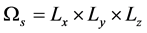 be a cuboid with side ratios either 4:4:1 for
  and 1:1:1 for
  with almost everywhere Lipschitz continuous boundaries
 . We are interested in the solution of the following problem:
Problem 1. For given values of ,
,  , find fluid velocity vector- function
  and scalar function of fluid temperature
  that satisfy the following:
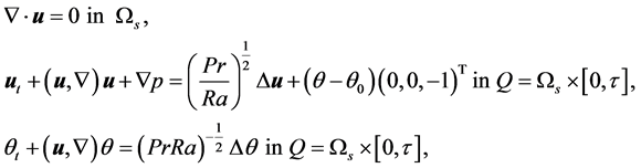 (1)
(1)
equipped with initial-boundary conditions:
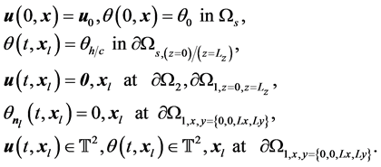 (2)
(2)
Here  is a solution on a 2D torus, i.e. periodic, in appropriate direction,
  -unit outward normal to the
  boundary,
  is the pressure;
 ,
,  are Prandtl and Rayleigh numbers, where
  is the magnitude of gravity;
  is the fluid thermal expansion coefficient;
  is the length in the direction of gravitational force (
 in our case);
  is the fluid thermal con- ductivity;
  is the fluid kinematic viscosity;
  is the temperature on the hot plane of the domain and
  is the temperature on the cold plane of the domain,
 . The nondenominational form is derived if the time scale is chosen as characteristic time for momentum transfer by viscosity through the layer of height
 . Pressure is not explicitly defined and is treated differently for every numerical method that we use.
3. Stability of the Main Solution
We are following [3] to show the analysis of stability for the main stationary solution. Considering a layer of fluid that is defined on  with
with  and boundary conditions of temperature set to
 ,
, . The boundary conditions for velocity
can be either set up as non-slip, i.e.  or free slip, i.e.
 . Setting
  in
in  we get
 , so
, so
the stability is defined for the linearly varying temperature profile with no dependence on . So we will consider the stability in the form of normal modes with fixed wave vector
 :
:
 (3)
(3)
where  is the increment and
  is the planar waveform function being a solution to the Helmholtz equation
 , i.e.
 with
with  and reality condition
  and
and
 , where
  is a complex conjugate. Solving (3) for
  one gets the following homogeneous equation [3] :
 (4)
(4)
Applying normal mode analysis to (1) gives the following boundary conditions for (4):
 (5)
(5)
The case for the free slip condition can be easily solved by choosing eigenfunctions in the form of  that satisfy boundary conditions. The solution of the quadratic equation for
  is:
is:
 (6)
(6)
for the case of stability loss  one can find that
and also see that the stability of the main solution is not dependent on . However coming up with eigenfunctions for the non-slip case is much harder so we use numerical approach, since we are only interested in the value for
  itself.
We seek solution for the critical point  in the form
 . Plugging con- ditions into (4), one gets:
 (7)
(7)
that has the following six roots:
 (8)
(8)
So the solution for  is presented in the form:
 (9)
(9)
The solution for the constants can be organized in the homogenoius system of linear equations using boundary conditions (5):
 (10)
(10)
where  is the column vector of the unknown constants A, B,・・・, F and matrix
  depends on the boundary conditions. We are not interested in finding
  explicitly, but rather determine the condition for the homogenoius liner system to have a solution and from that condition derive critical values of
  and
and , called
  and
and , respectively. For the free-slip boundary the expression for the matrix is:

corresponding to , row wise. For non-slip boundary conditions the matrix is:

corresponding to 
 , row wise. The determinant of
  must be zero in order for the system (10) to have a nontrivial solution. So for a fixed value of
  we must solve the nonlinear equation
  numerically. It is done by using Newton method as:
 (11)
(11)
here the Jacobi matrix is found using analytical differentiation technique. Iterations stop if . On the other hand, knowing from the literature [3] the critical values of Rayleigh number, one can find a critical wavenumber
  using the same method for fixed
 . It should be noticed, however, that the solution should be pure real despite that the roots are complex. In Figure 1 we show neutral curves for

Figure 1. Neutral curves for free-slip and non-slip boundary conditions. Dot plots are numerically calculated points of first bifurcation for given  and non-slip boundary conditions for
 . Asterisks for Fourier-Galerkin method and circles for Finite Element/Volume Method.
both cases of boundary conditions with  and
and . So one can verify the appearance of the first bifurcation in numerical methods.
4. Numerical Methods
In this section we give information about numerical methods that are used to solve the problem.
4.1. Pseudo-Spectral-Galerkin Method
The Pseudo-Spectral-Galerkin Fourier-Chebyshev method is applied to the domain  (Fourier-Galerkin method or FGM for short). All vector-functions in (1) are expanded by the divergence free basis functions
 , constructed analogues to [5] :
 (12)
(12)
We can check that the following bases functions are analyticaly divergence free, i.e. , no matter the expressions for them. For the case of
  we use the following set of scalar bases functions:
 (13)
(13)
where . We use Chebyshev polynomials in
  direction for
 , as in [5] for 2D and 3D Dirichlet box cases. We use the relation for Chebyshev polynomials of the first and the second kind to get:
 (14)
(14)
In order to meet homogeneous Dirichlet conditions we must have:
 (15)
(15)
With all this together we get the following scalar basis functions in  direction:
 (16)
(16)
It is a straightforward way to check that (16) and, hence, (12) are complied with (14) and (15). Such functions form a basis in  that we use to approximate the solution of the initial-boundary value problem (2) for (1). Note, that the basis (12) is not orthogonal in
  direction but orthogonal in
  directions due to the use of Fourier basis functions. It can be shown by the construction of the Mass matrix using an
  projection.
From here we turn our attention to the truncated series for basis functions, so that the problem can be solved on the computer. We assume that there are  number of polynomial modes, i.e.
  is the number of Fourier modes and
  is the number of Chebyshev polynomials in
  direction. Please note that the number of degrees of freedom is lesser since all complex coefficients for Fourier modes are subject to reality condition, i.e.
 . So the total number of degrees of freedom is
 . In this case the basis scalar components (13) are rewritten as:
 (17)
(17)
Since the basis is divergence free and the mean flow through periodic boundaries is zero, this implies that the integral of velocity over these boundaries is zero. In this case it is straightforward to show that the pressure is eliminated from (1) by projecting pressure gradient into the divergence free functional subspace that is formed by the span of divergence free basis functions.
We use the following scalar basis functions for the temperature expand:
 (18)
(18)
where  are constructed such that boundary conditions for temperature are satisfied:
 (19)
(19)
With the correction term  we satisfy boundary conditions for temperature
on .
.
The cost of the full Bubnov-Galerkin method being applied to Equation (1) is of  due to the non-linear term. These multiplication terms become con- volution in the functional space thus causing multiplications of tensors rank 3. Such computation complexity is very limiting. In order to reduce the computational cost of calculations we use two stage transfer from physical space to functional space and use Fourier collocations with pseudo-spectral approach in
  direction.
First we span the functions in (1) using Discrete Fourier Transfer (DFT) in regular grid points, forming the following system (taking into account divergence-free nature of basis):
 (20)
(20)
with  being a convolution term. All coefficients
  with
with  being DFT coefficients.
For every  point we apply Bubnov-Galerkin projection in
  direction:
 (21)
(21)
where we denote:
 (22)
(22)
 (23)
(23)
as projections of DFT basis corrected coefficients to polynomial space and ,
,  ,
,  ,
,  are mass and diffusion matrices for velocities and temperature, respectively for every point
 . Matrix sizes are
  and they are formed as:
 (24)
(24)
 (25)
(25)
 (26)
(26)
 (27)
(27)
where  and minus sign in diffusion matrices is due to the in- tegration by parts and zero boundary conditions. Since these matrices are independent of
  indexes, we can apply them for each point
  in
in  -direction. The mass matrices are full since the basis we use is not orthogonal but all matrices are not singular. It can be proved by the fact that we are using linear combinations of polynomials that form basis in
 . So the vectors are linear intendant and so the matrices are positive-definite, hence, invertible and the system can be solved for unknown coefficients
 ,
, . In order to perform integration we use exact symbolic integrals for diffusion and inverse mass matrices that are calculated in Wolfram Mathematica and stored for further use in the program. We use Gauss- Chebyshev quadrature in
  direction. This quadrature is exact for polynomials of degree
  and can be efficiently used. We use it to perform projection from domain to image and back for (22), (23) and we find DFT divergence-free coefficients at points
  as
as
 (28)
(28)
 (29)
(29)
where  points are Gauss-Chebyshev quadrature points and
 ,
,
where  so boundary points belong to the boundary.
The nonlinear (multiplication) term is calculated using pseudo-spectral approach. We calculate derivatives in polynomial space, then return to the physical space at specific points and calculate multiplication in physical space with computational difficulty . Having known coefficients
 ,
,  at time
  we perform the following steps to calculate
  (the advection term in scalar energy equation is calculated analogously).
1) Calculate derivatives in functional spaces:
 ,
,  ,
,  ,
,
where  is the differentiation matrix for our basis functions in
  direction.
2) Increase the size of arrays for  and
and  in
in  and
and  direction by
  and fill added elements with zeros, so we have arrays with sizes of
 .
.
3) Return from functional space to physical space step by step to get  and
and :
:
・ use (28) for every  and
and  to get
 ;
;
・ Apply inverse DFT for every plane at .
.
4) Calculate multiplication in physical space at every point to get:
 .
.
5) Return back to Fourier space using DFT for every plane in . Truncate series to the size
  by removing modes that are padded by zeros earlier to get
  and
and .
.
6) Apply (22) using Gauss-Chebyshev quadrature to get  where
where ,
,  and
and .
.
This leads to no aliasing of frequencies.
The following approach requires less operations then the exact Bubnov-Galerkin method of  [9] . The most operation-hungry part is the nonlinear term calculation using 3/2 padding. Now we assume that FFT can be used for DFT with
  operation, for example one can use fftw or cufft on GPU. Calculation of derivatives is done using
 . We need
  ope- rations to perform DFT, then we need
  operations to get transfer in
  -direction. Multiplication in physical space requires
  operations. And return to the image from the domain of the mapping requires the same difficulty as for the image to domain transfer. So we get maximum difficulty as
  , and for most practical use (say
 ) the limiting factor would be
  so we assume that our method requires
  operations for every time step.
Explicit Runge-Kutta 4 (RK-4) method that is used to integrate the semi-discrete system (21) in time. In order to satisfy stability condition we analyze spectra of the linear operator and bounds for the nonlinear part and derive stability condition. A necessary condition for stability by the linear change of mapping (by the change of the time step) is the location of all discrete spectra of the spacial operator inside the RK-4 stability region on a complex plane. The discrete Fourier spectra has a standard estimate [9] and spectral norm for Chebyshev matrices is used for the estimate. This part is beyond the scope of the paper.
4.2. Finite Element/Volume Method
We consider another method that is applied in  and
and  domains. It uses nodal Finite Element approach to reconstruct pressure and Finite Volume/Difference method for the reset part of the equations. Finite element method uses values of pressure and velocity in vertexes of elements to form matrix equations. Finite volume/difference method uses values of velocities in centers of elements to approximate integral/ differential operators. So this is a combination of finite element method and finite volume method that we call “FEM” for short.
We start with discretization of Stokes operator:
 (30)
(30)
in bounded domain  with appropriate initial-boundary conditions. We use some discretization method that we discuss later and projection method (see [10] ) to translate (30) into:
 (31)
(31)
Here  is a mass matrix;
  is a gradient matrix;
  is a diffusion matrix and
  is a divergence matrix. We introduce time slices with
  being
being  -the time slice with time-step
  and derive the following system:
 (32)
(32)
Since  is unknown on
  -th time slice, we split the system as:
 (33)
(33)
and introduce velocity correction vector  and scalar potential function
 :
:

hence:

so , and we get correction equation for the potential function
 :
:
 (34)
(34)
where matrix  is a Schur complement. After the solution of (34) we correct velocity and pressure functions in such way, that
 :
:
 (35)
(35)
where  is a parameter. This projection method is another way to write Helmholtz-Hodge decomposition for specific type of equations. The whole step of solution consists of using three steps (33), (34), (35). In general this results in first order of approximation for (30) in time. The stability and consistence of the method depend on the discretization. It is known that the discretization must obey Ladijenskaya- Babuska-Brezzi (LBB)
  condition in order to be stable and consistent. In case of the provided approximation it means that
  (corre- sponds to
  condition) and that
  (corresponds to
  condition), where
  is a condition number and
  is a discretization parameter (e.g. grid size). In general one usually takes
 , chooses mixed finite element ap- proximation (for finite element methods) or staggered grid (for finite difference approximation) and changes matrix
  to
to  that can be easily inverted, e.g.
 . Here we use different strategy that is dealing with different approximations for different operators.
Let us introduce rectangular cuboids  that from a 3D tessellation of a rectan- gular domain
 , such that
 , where
  is a multi index with
  being a center of
 . We introduce another set of tessellation
  that is constructed from swapping central nodes and vertexes, thus each vertex of
  becomes a center for
  and vice versa.
We define basis functions in an element , where
  can be
  or
or , as follows:
 (36)
(36)
Now we use the following expansion in this element space for a scalar function :
:
 (37)
(37)
Now we consider set of points  formed by the centers of
  or vertexes of
 .
.
Such elements can be considered as finite volumes, i.e. . We now
define the following differential operators:  and
and  in space of nodal finite elements
 ,
,  and
and  in space of finite volumes
 , we use Laplace operator
  for the approximation of
  and identity matrix for
  and
and . Define projection of nodal operator to central finite volume point as
  and projection of central finite difference/volume operator to nodes as
 . The first operation is performed using (37) with
  and the second operation is an inverse of (37) with
 . In this case the scheme can be written as follows:
 (38)
(38)
In this work we use compact finite difference scheme of 4-th order to approximate  and
and  using method of alternating directions. The approximation of
  and
and  is done using Bubnov-Galerkin projection (integration over
 ), e.g. for the second equation in (38):
 (39)
(39)
Inserting (37) into (39) and doing integration by parts:

where ,
,  are coefficients of expansion for Dirichlet and Neumann boundary conditions and
  are coefficients of divergence operator projection into the space of finite elements. Other operators are derived analogously.
It is a straightforward way to check the BBL condition (we don’t consider this in the papaer). Trivial kernel of  and
and  is proved by considering space of finite elements and 4-th order compact differences schemes. The condition number of finite element approximation can be estimated from the space of finite elements and can be shown that it has a marginal bound. Now it is a straightforward way to return to Navier-Stokes equations by applying some approximation for the nonlinear term in (38) (defined bellow as
 ). We use 7-th order WENO scheme that has good spectral properties and guaranties TVB behavior of the solution (on each WENO stage we use Runge-Kutta 3rd order SSP method [11] ). In order to increase the temporal accuracy we also use Runge-Kutta 3rd order explicit method [11] for which the projection step (38) is applied on every stage. The stability of the method is deduced from CFL condition since diffusion is considered in implicit way. The usage of this type of finite elements gives one more positive result. There is no artificial boundary layer near wall boundary. Equation on
  requires zero Neumann boundary conditions on the wall, but in this FEM setup it just means skipping values of
  on zero Neumann boundary. The same is true for the pressure gradient approximation. Then the total scheme for (1) is given as:
 (40)
(40)
 (41)
(41)
4.3. Solution of the Eigenvalue Problem
We briefly give description of the matrix free eigenvalue solver that is used for the problem. More information about this approach can be found in many papers, for example [12] [13] [14] [15] . Considering discrete systems (21) and (41). Let us consider another discrete systems for small temporal perturbations  and
and  formed in the vector:
 (42)
(42)
Inserting those into discrete systems and linearizing one can gets the following set of equations:
 (43)
(43)
where
 (44)
(44)
where


for Fourier-Galerkin system and
 (45)
(45)
for FEM system. Here  stands for linearization of the operator (40). The size of the perturbation vector is
  and is used in the Implicitly Restarted Arnoldi (IRA) method. Note that if we are using Fourier method, this vector includes real and imaginary parts of Fourier modes that are treated as real values and the size changes to
 . The system (43) is used as an operator
  that maps the vector (42) as
 . These perturbations are automatically divergence-free since we are using divergence-free basis for Fourier-Galerkin method. For FEM method these perturbations are guaranteed to be divergence-free since we are applying projection algorithm with pressure initialized during the projection. There’s no need to introduce pressure perturbations in both cases. The algorithm for IRA to find eigenvalues of
  is based on [16] and goes as follows:
1) Initialization. Initialize vector  with different random values. Then normalize the vector, so
 . Select number of eigenvalues
  that are desired and number of additional vectors
  for the implicit procedure, so the dimension of Krylov subspace is
  and we set variable
  and vector
  which are defined later.
2) Arnoldi Step. We form the Krylov subspace as  where
where  and
and . We use the following process:
if  equals to 0 do
a) ,
,
b) ,
,
c) ,
,
d) Gram-Schmidt process correction: , until
 ,
,
e) , where
  is an upper Hessenberg matrix and
 ,
,
continue

a) ,
,
b) ,
,
c) ,
,
d) ,
,
e) ,
,
f) Gram-Schmidt process correction: , while
 ,
,
g) .
.
This precess generates the following decomposition:
 (46)
(46)
 : the last vector after the application of step 2,
 . If the last value
 , then vectors in
  are linearly dependent and
  is invariant under the application of
 . The process stops with
  and eigenvectors (eigenvalues) of
  are the eigenvectors (eigenvalues) of
 . If the process is not stopped (which is usually true), then continue to 2. Find eigenvalues of Hessenberg matrix
 , sort them in an appropriate order (either maximum real part or maximum magnitude in our applications). Perform QR algorithm with shifts for H using polynomials with number of shifts
 :
:

a) ,
,
b) .
.
Set . Note that at this point
  since some of
 . Apply shifts:
 ,
,  ,
,  ,
,
 ,
,
 ,
,
 .
.
At this point we have matrices ,
,  with additional value
  and let
  be an eigenvalue of
  with associated normalized eigenvector
 . We denote
  as a Ritz vector of
  and Ritz value
 , both associated with
 . For these Ritz variables we have [16] :
 , where
  is the last component of the
  eigenvector. So, while
 , goto 2.
In order to find eigenvalues of Jacobi matrix we consider the system (43) with zero temporal derivative. So the system (43) is called on every stage of Arnoldi process by applying the linearized equations to the vector in Arnoldi step. If we are computing eigenvalues of Monodromy matrix then the system is applied as follows. Let the system (43) have a periodic solution with period . Then the system is formed as
 (47)
(47)
where  is a state transition operator or a Monodromy matrix. To find
  in a matrix-free way we integrate the linearized system in time for a period
 :
:
 (48)
(48)
so,
 (49)
(49)
Now we apply (48) for the input vector in Arnoldi step of IRA, while integral is evaluated by applying the selected time stepper.
4.4. Implementation Details
Our goal is to perform direct numerical simulation (DNS) of problems and trace transition from initial stationary point in the phase space (main solution) to the chaos through cascades of bifurcations. In order to detect and clarify bifurcations we use the analysis of eigenvalues of Jacobi and Monodromy matrices and phase portraits with Poincare sections. The calculation of the whole IRA algorithm and achievement of the statistically quasi-periodic solution regimes for relatively high  numbers require significant computational power. We use the same idea as in [8] to adapt number of harmonics or number of elements for the problem during the analysis of bifurcations. The control of the accuracy is done by the analysis of the energy spectrum for the whole simulation time. We define the correlation tensor
 (50)
(50)
and its Fourier transfer
 (51)
(51)
For the discrete problem we are using FFT to calculate (51). In order to get the energy spectra we integrate over the spherical shell:
 (52)
(52)
that becomes a summation for the discrete problem. Then we check, that for :
:
 (53)
(53)
with  being the size of FFT discretization. The last relation (53) in physical interpretation means a track of the solution to be in a deep dissipation regime. It is an overdiscretization from a standard DNS point of view, however it is essential to obtain complex bifurcations in near chaos region. For all calculations we are using
 ,
,  modes for Fourier-Galerkin method and
  elements for FEM method in
  domain and
  elements in
  domain. During the IRA process we find 6 or 10 leading eigenvalues (i.e.
 ) and use 94 or 90 additional Krylov basis vectors, so
 , and
, and , thus
  and Hessenberg matrix size is
 .
.
In order to accelerate computations we are using multiple Graphic Processor Units (multiGPU). The GPUs used are k40 NVIDIA GPUs, all programs are implemented on C++ with CUDA C. The application of DFTs is done by the CUFFT library on 2 or 4 GPUs. The matrix vector products are conducted using MAGMA library. The solution of the Poisson Equation (39) is carried out using geometric multigrid approach [17] . The IRA algorithm is using dot product, matrix-vector operations and matrix matrix operations from MAGMA library across multiGPUs, wheres QR routine for the upper Hessenberg matrix is taken from LAPACK. The visualization is done using GMSH [18] , Gnuplot and LibreOffice, simple calculations are done in MATLAB.
5. Benchmarks
At first we perform the verification of our methods vs. known results. The first benchmark is to obtain the neutral curve by applying different  as it is done in Section 3. For this purpose we consider domain
  with the following perturbations of temperature:
 (54)
(54)
where  is a given critical wave number, and we take
 . The results for numerical methods are brought in Figure 1 with comparison to the linear stability analysis. We can see that maximum deviation for FEM (
 elements) method is about 11.2% and for FGM is about 6.5% (
 modes). Please note that further increase of degrease of freedom did not improve the results much. We are able to trace exact points of transition with the application of the IRA solver. The results for leading eigenvalues are brought into Table 1. Please note that for both cases we have leading eigenvalues of multiplicity two. So the supercritical pitchfork bifurcation is observed, that complies with well known data about Rayleigh-Benard convection. In physical space we can observe the formation of rolls that run parallel to one of the axis
  or
or , depending on the direction of perturbation vector in (54). Velocity vectors for these rolls are shown in Figure 2. One can observe small amplitude of velocity but the amplitude increases with the increase of
 , with the formation of a mushroom type distribution for temperature.
Velocity vectors and temperature distribution for  are shown in Figure 3 for
  obtained with
  elements using FEM. The critical pertur-

Table 1. Leading eigenvalues for the first bifurcation for four critical wave numbers.

Figure 2. Velocity vectors and temperature distribution in  for FGM with
 , using
  modes. (a)
 . (b)
. (b) .
.

Figure 3. Velocity vectors and temperature distribution (with cross section) in  for FEM with
 , using
  elements. (a)
 . Velocities. (b)
 . Temperature iso-surfaces and horizontal section.
bation was chosen as  and interpolation in Rayligh number values using results from eigenvalue solver give
  for this problem. We can check these results with data from [4] where
  is presented. One can see that the presented eigenvalue solver with numerical methods correctly represents first bifur- cation.
Another benchmark that we are running is a DNS data comparison with data, available at [19] and more information can be obtained at [20] . We are not using eigenvalue solver since the regimes for this DNS are in turbulent regime and it corre- sponds to multiple unstable eignevalues for non stationarity solution. For the DNS ben- chmark we are using the same setup as in [19] , namely  with
with . Random initial perturbation for temperature is used. For this benchmark we are using FGM with
  modes and FEM with
  elements. Since the flow is in deep turbulent regime, we are calculating statistical data:
 ―mean spacially averaged values;
 ―root mean square values;
 ―total kinetic energy of turbulence and
 ―total dissipation of turbulent kinetic energy, that are defined as follows:

here  is an averaged Raynolds number taken analogous to [20] for the considered problems,
  is a Reynolds averaged data,
  is an fluctuation data,
  is a period of averaging that is taken equal to [19] as 20 time planes, each
  ensembles for FEM method and analytical space integrals for FGM method.
Instantaneous snapshots of temperature distributions are shown in Figure 4 and Figure 5. Note that for the latter distribution the boundary layer is thinner. Com- parison of statistical characteristics with available data from [19] is shown in Figure 6. It is clear that the statistical data is close to the provided simulation data. Please note, that the current results are obtained with higher order methods and, thus can be more exact. But in general the distribution is similar and so one can conclude that the proposed numerical methods for relatively hight Raylight numbers are correct. The leading direction of the flow is determained by the initial perturbations. In order to compare results with [19] we used  -dominated perturbations.

Figure 4. Instantaneous temperature distribution in  domain for air, results from FEM method. (a)
 . Temperature iso-surfaces. (b)
 . Temperature iso-surfaces with inclined plane cut.

Figure 5. Instantaneous temperature distribution in  domain for air, results from FEM method. (a)
 . Temperature iso-surfaces. (b)
 . Temperature iso-surfaces with inclined plane cut.

Figure 6. Comparison of statistical data for different . (a) RMS velocities,
 . (b) Total kinetic energy and total dissipation of turbulent kinetic energy,
 . (c) RMS velocities,
 . (d) Total kinetic energy and total dissipation of turbulent kinetic energy,
 .
.
6. Bifurcations and Route to Chaos
Some bifurcations for the problem in  were presented in [8] as a survey of the results with the main emphasis on the Feigenbaum-Sharkovskiy sequence of cycles. In here we give new results for both setups.
6.1. Bifurcations in Domain with XY Periodicity
After the first bifurcation that is shown in Benchmarks section the flow stays steady that corresponds to the point in the phase space that remains in this point for  with gradual increase of velocity amplitude. At around
  for FGM and
  for FEM, leading eigenvalue with multiplicity two crosses the imaginary axis. This results in another supercritical pitchfork bifurcation, forming solution that is symmetrical in another plane. Velocity vectors and temperature distribution are shown in Figure 7. We can see that the solution is now rotated
  with the formation of similar rolls.

Figure 7. Velocity vectors and temperature distribution in  for FGM and leading eigenvalues of Jacobi matrix near Andronov-Hopf bifurcation at
 . (a)
. (a) . (b)
. (b) . (c) Leading Jacobi matrix eigenvalues.
The Andronov-Hopf bifurcation occurs near  for FGM method and around
  for FEM with the formation of limited cycle in the whole phase space. The following process for FGM is depicted in Figure 7. The limited cycle increases its amplitude and for
  is shown in Figure 8 alongside with the eigenvalues of Monodromy matrix. The corresponding velocity and temperature distributions are shown in Figure 9 and trajectories in physical space with the magnitude of leading eigenvector are shown in Figure 10. It is clear that one eigenvalue is located at the unit cycle at the point
  that corresponds to the limited cycle. It is true for both numerical methods, although the convergence of IRA is faster for FGM method. Other eigenvalues are situated inside the unit circle and are stable. One can see the difference in eigenvalues for FEM and FGM methods, however both methods give correct leading eigenvalue. As one can see from the eigenvector, the flow is formed by the bending of the rolls with the subsequent oscillation. Although the attractor dimension is just one (limited cycle), the flow in physical space is already complicated. It can be traced with the stream lines obtained by Lagrangian particle tracers (Figure 10) that are forming a complected path in the physical space.
At this point one may observe the effect of multistability. If perturbations of magnitude  are applied to the system, the solution drifts to another attractor of dimension zero, i.e. stable point, temperature and velocity distributions are shown in Figure 11. It is clear that a formation of distorted square structures is presented. If we trance this solution back by decreasing
  we will get the square tile structures. For

Figure 8. Cycle projection and ten leading eigenvalues of Monodromy matrix for different methods, . (a) Projection of cycle to three dimensional phase subspace. (b) Eigenvalues of Monodromy matrix.
further reference we are not paying attention on multistable solutions near our main branch unless they form different scenario of transition to chaos.
With the further increase of  number we see the increase of amplitude of the limited cycle and with the sequential formation of the invariant two dimensional torus. It can be expected since complex-conjugate eigenvalues of the Monodromy matrix in Figure 12 are closing to the unit circle on the complex plane. In order to obtain these results we had to run IRA with the same randomly initialised vector for all values of
 . Secondary Hopf bifurcation occurs at
  for FGM and
  for FEM. This leads to the formation of the limited torus in the phase space, whose projection into three-dimensional subspace is shown in Figure 12 and physical space functions are shown in Figure 13. Please note that in many papers the bifurcation that leads to the formation of invariant torus is called Neimark-Sacker bifurcation. This is a

Figure 9. Instantaneous velocity vectors and temperature dis- tribution in  for FGM. (a)
 . (b)
. (b) .
.

Figure 10. Lagrangian particle movement in  and magnitude of leading eigenvector that corresponds to maximum magnitude eigenvalue of Monodromy matrix, located at
  on the complex plane for FGM. (a) Lagrangian particle movement. (b) Modulus of the leading eigenvector for velocities.
misuse of the term, since Neimark-Sacker bifurcation occurs in generic dynamical systems generated by iterated maps, see [21] , p. 113. Since we consider discrete system

Figure 11. Multistable solution for  at
at  for FGM. (a)
  temperature isosurfaces. (b)
  velocity distribution.
 (a)
(a)
Figure 12. Leading eigenvalues of Monodromy matrix near second Hopf bifurcation as functions of  and 2D invariant torus in phase subspace. (a) Evolution of Monodromy matrix leading eigenvalues. (b) Projection of invariant 2D torus into three-dimensional phase subspace.

Figure 13. Temperature and velocity distributions in  for
for  that coresponds to the invariant torus in the phase space. (a) Velocity vectors. (b) Temperature isosurfaces.
that approximates continuous one and use high order methods we assume that the behavior of our discrete system is close to the continuous one at least as long as the estimate (53) holds. So we use the term secondary Hopf bifurcations for such bifurcations that have simple complex conjugate eigenvalue with zero real part at the critical point in parameter space and lead to the increase of the attractor dimension by one.
With the increase of the  we can observe the formation of the 2D invariant torus with period two that can be traced through the analysis of Poincare sections only. The period doubling bifurcation takes place at around
  (for both FGM and FEM) on the second frequency (the corresponding eigenvalue crosses unit circle at point
 ). Results of the phase space projection and Poincare section are shown in Figure 14. With the further increase of
  a resonant torus is formed it can be observed on the same figure in the Poincare section for
  using FGM. Such exact value was chosen in order to perform eigenvalue analysis (was found using quasi-Newton method). The period during integration
  in (48) was defined by the return map in the Poincare section. Please note that the calculation of these eigenvalues took about a month on a 5GPU cluster. Corresponding eigenvalues are presented in Figure 15. Two pure real eigenvalues have magnitude close to unity (0.999 and 0.997 and we assume that these eigenvalues are of magnitude one) and are located at the
  point on the unit circle. This is another way of saying that the system has two zero Lyapunov exponents and all other exponents are negative (inside the unit circle on the complex plane). This corresponds to the phase-lock of three frequencies: two are connected through period doubling and another was irrational to them both. It is interesting that there are two more eigenvalues are closing the point
  that can mean a possibility of period doubling bifurcation. However with the increase of
 , after the phase-lock, the system continuous to maintain the same attractor (2D two period torus with increasing magnitude) and suffers anther phase-lock (with another frequency of the period doubling) at about
  (see Figure 15). Again, two pure real eigenvalues are of unit magnitude (1.019 and 0.998) correspond to zero Lyapunov exponents. However there are more eigenvalues closing to the unit circle in

Figure 14. Invariant 2D torus period 2 and Poincare section for it with close resonant torus. (a) Projection to the three dimensional phase subset, . (b) Poincare section using plane
 ,
,  and
and .
.
this case.
From this point the solution branches dramatically. The first branch is presented by the solutions with no perturbation introduced. In this case the solution undergoes the formation of hyperbolic attractor on one of the torus cycles starting from . Please note that we present data only from FGM here since FEM was not used for this branch. Evolution of return maps is shown in Figure 16. One can see that the onset of chaos emerges very fast in parameter space through local hyperbolicity. With this the attractor dimension remains bounded between 2 and 3. This can be stated since the

Figure 15. Leading eigenvalues for resonant 2D torus period two in two cases of phase locking. (a) Leading eigenvalues of the resonant torus, . (b) Leading eigenvalues of the resonant torus,
 .
.
second Poincare section (Poincare slice) is void. In order to justify the fact of local hyperbolicity let us consider a zoom-in of Poincare section for  and construct series of Lameray diagram. In Figure 17 we show a part of Poincare section (we selected the one that is closer to the straight line located at
 in Figure 16) that was rotated in such way that the image of the mapping is of minimal width. Then for this data we construct

Figure 16. Transition to chaos through hyperbolic attractor on a 2D invariant torus period two. (a) Poincare sections for different  (resonance),
  ,
,  ,
,  ,
,  (chaos). (b) Projection into three planes of a 3D Poincare section for
 .
.
Lameray diagram by considering mapping , where
  is
is  data in selected Poincare section part. One can see that the iteration map has neither cyclic behavior (as can be exacted in case of finite number of period doubling bifurcations) nor convergence. If we take more data the points on middle figure (Figure 16) will

Figure 17. Analysis of Poincare section fragment for . (a) Rotation of Poincare section fragment. (b) Lameray diagram for mapping
 . (c) Action of Lameray mapping.
form a fractal set with infinitely many close inclusions. Examples of such maps for ODEs are constructed in [22] . However we may assume another scenario of fast and multiple period doubling bifurcations with the formation of singular Feigenbaum attractor in the Poincare section. This can be implied through the analysis of some leading eigenvalues that are located closer to the  point for resonance case, see Figure 15. But for this case (close to the resonance) the IRA algorithm filed to converge so we cannot justify this scenario. We are unable to reveal any localized structures for
  in the phase space for this branch.
Another branch is observed if small perturbations (of  magnitude) were introduced at
 . In this case the system turns itself to another torus solution that further undergoes secondary Hopf bifurcation with the formation of a 3D invariant torus at around
  for FGM and
  for FEM. First and second Poincare sections are shown in Figure 18 that were obtained using FGM.
This 3D invariant torus remains stable for the whole calculation time (up to 60 mln time steps) and for  (8654 for FEM) we can observe a possible formation of a 4D invariant torus, see dynamics of its formation in Figure 19 for
 ,
, . Please note that these results were obtained on FGM with increased spacial resolution up to
 . One can see on the spectra of the signal (Figure 18) that there are more frequencies in the low wavenumber region for 4D torus regime. This possibly can be explained by the reverse energy cascade pumping from high wavenumbers due to the decrease of diffusion. The solution becomes chaotic for
 . Thus an initial stage of Landau-Hopf scenario is found in this branch with the formation of attractor dimension at least four.
Another branch can be found by the application of the symmetric initial conditions for . We are using
  and first bifurcation takes place at
 . In this case the flow is formed by roll structures (Figure 20) through the first supercritical pitchfork bifurcation that remain in the same direction without the second pitchfork bifurcation. This branch can be traced only by FGM because FEM drops to one of the “tori” solutions with distorted roll structures that were discussed above. A a consequence a solution tends to preserve symmetry and this branch is developing through bifurcations of limited cycles. The amplitude of velocity grows with the increase of
  and at
  the solution has an Andronov-Hopf bifurcation that leads to the formation of the limited cycle.
Eigenvalues of the Jacobi matrix, Monodromy matrix and cycle projection into phase subspace are shown in Figure 21. Monodromy matrix has one real eigenvalue at  on the complex plane that corresponds to one zero Lyapunov exponent, thus forming a limited cycle in the solution space since all other eigenvalues are inside a unit circle. One can see that two more eigenvalues are approaching
  point that indicates period doubling bifurcation. It takes palace at
  with the formation of limited cycle period two. The full bifurcation diagram is presented in Figure 22, the idea of its construction is taken from [6] . We will not stop on detail analysis of every solution and only point out that further increase of
  leads to the

Figure 18. Transition to chaos through the Landau-Hopf scenario. (a) Phase subspace and Poincare sections for . (b) Poincare section for
 . (c) Time series spectra for
 .
.
development of full Feigenbaum-Sharkovsky inverse and direct cascades. However, due to multistability we observe formations of cascade threads. For example, at around

Figure 19. Transition to chaos through the Landau-Hopf scenario-formation of 4D torus. (a) Second Poincare sections for  that corresponds to stable 3D invariant torus. (b) Second Poincare section for
  and
and .
.
 we have another multistable solution that has cycle period two. Another multistable solutions are observed at
  and
and  that are presented by cycles. At some points the solution has an effect of intermittency (for example at

Figure 20. Roll structures for symmetric branch, stationary solution. (a) Velocity for symmetric branch, . (b) Temperature for symmetric branch,
 .
.
 and
and ). Example of such intermittency is presented in Figure 23 along with cycle period three from Sharkovsky cascade and its Monodromy matrix eigenvalues. Finally the system emerges into chaos through singular attractor and from
  we are unable to detect any regular structures in the phase space.
6.2. Bifurcations in Bounded Cubic Domain
We are only discussing results here that were not mentioned in [8] . This subsection is focused on eigenvalues since we were unable to perform eigenvalue analysis in our previous papers due to computational limitations. All results are obtained with FEM.
There were three series of experiments conducted in [8] for various  numbers. Each series resulted in different scenarios of transition to chaos. As a matter of fact, this was not only due to
  change, but also due to the symmetries in the system. At first, all scenarios have a common initial stage-supercritical pitchfork bifurcation. The first one was found in Section 5. The Rayleigh number of all bifurcations is higher compared to periodic domain due to the wall stabilization effect. If the initial perturbations are given as discussed in Benchmark Section 5 (dominated along one of the axis), then the flow develops a symmetrical solution in one plane, see Figure 24.
Another set of initial conditions may lead to other symmetries. For example, corner structures are formed if an initial condition are taken with constant perturbation of magnitude  in the form:
 (55)
(55)
where  is taken to have equal area. Results for
  are presented in
Figure 25. These solutions are symmetric relative to planes: .
.
The direction of symmetry is selected only by initial conditions. Further increase of  number leads to the increase of amplitude of velocities. Finally, the solution can either go through supercritical pitchfork bifurcation or through Andronov-Hopf bifur-


Figure 21. Jacobi and Monodromy matrix eigenvalues and projection of the limited cycle. (a) Leading eigenvalues of Jacobi matrix for different . (b) Limited cycle projection into phase subspace,
 . (c) Leading eigenvalues of Monodromy matrix,
 .
.

Figure 22. Bifurcation Diagram for symmetric branch.  is a projection of middle plane section to
  -axis. Two points indicate a cycle, four-cycle period 2, discrete set of points-singular Feigenbaum or Sharkovsky cycle, line-chaos.
cation without the pitchfork (for example see Figure 26). Solutions are asymmetric in  in the first case and this leads to the multiple invariant tori bifurcations, see [8] . In the second case the solutions are symmetric relative to a plane (e.g.
  in Figure 24) and this leads to bifurcations of limited cycles with the formation of singular attractors. It was noticed in [8] that the solution may become asymmetric while on a cycle cascade which leads to chaotic solution through subcritical pitchfork bifurcation. It can be seen by the analysis of the Monodromy matrix eigenvalues in Figure 26. Eigenvalues closer to
  point are responsible for possible future period doubling bifurcations, but an eigenvalue closer to the leading one at
  can be responsible for secondary pitchfork bifurcation.
We present an example of a symmetric singular attractor in Figure 27 for  . Note that Poincare section of the attractor is perfectly symmetrical in
  plane, but asymmetric in
  plane (in this particular case the section is symmetric relative to a central point). Another example is the formation of a singular attractor from Sharkovsky cascade cycle of period 3 that is shown in Figure 28. We are able to analyze eigenvalues of Monodromy matrix for the cycle period 3 (C3) for
  and for a small deviation from the parameter value. One can see that for C3 all eigenvalues are inside the unit circle except for one at
  point. With the increase of
  we can observe that seven leading eigenvalues out of ten are escaping the unit circle through the point
 . Please note that these seven eigenvalues are scaled down to fit on graph. Maximum magnitude of the first eigenvalue is 23. This justifies the fact that the singular cycle (shown in Figure 28) is developing through series of period doubling bifurcations. After these singular cycles we are unable to detect any structures in the phase space.
7. Discussion
There are more questions to discuss that are not touched here. The problem of inter-

Figure 23. Intermittency and Sharkovsky cycle period three. (a) Inter- mittency at . (b) Projection of limited cycle period three,
 . (c) Monodromy matrix eigenvalues for
 .
.

Figure 24. Symmetrical solutions in plane  for
for . (a) Temperature dis- tribution. (b) Sections of temperature distribution. (c) Sections of velocity magnitude dis- tribution.

Figure 25. Symmetry solutions for modified velocity initial conditions at . (a) Temperature distribution. (b) Sections of temperature distribution. (c) Sections of velocity magnitude distribution.

Figure 26. Eigenvalues of Jacobi matrix for pitchfork and Hopf bifurcations and Monodromy matrix for . (a) Hopf bifurcation at
 . (b) Pitchfork bifurcation at
 . (c) Monodromy matrix eigenvalues.

Figure 27. Singular attractor phase subspace projection and Poincare sections for . (a) Cycle projection into 2D phase subspace. (b) Poincare section using velocity. (c) Poincare section using velocity and curl.

Figure 28. Cycle period 3 and singular attractor phase subspace projections, Poincare section of the singular attractor and eigenvalues of Monodromy matrix. (a) Cycle period 3 projection into 2D phase subspace for . (b) Singular attractor projection into 2D phase subspace for
 . (c) Poincare section of the singular attractor. (d) Evolution of Monodromy matrix eigenvalues.
mittency was only confirmed but not discussed in detail. It is a future work to confirm the ideas about the cubic mapping , to describe intermittency, as suggested in [7] . The dependence on
  was not investigated, how- ever it is known, see [7] , that the route to turbulence depends on it and intermittency emerges more for high
  (spacial instabilities are more elaborated in this case). The emergence of a 4D torus in Landau-Hopf scenario is still a question. It can be confirmed by the author’s new idea (to be published soon) of constructing an
  -net of splines over the attractor and tracking its evolution on the attractor. If the structure in question is a torus and its mapping in phase space is diffeomorphic, then the
  -net will converge. But it requires enormous amount of computational power and time. Another question is the automatization of the process of bifurcation detection and eigenvalue analysis as it was suggested in [12] [23] . Another question is the emergence of traveling waves for periodic problem and explicit study of it’s influence on bifurcation scenarios. All these questions are topics for further research.
8. Conclusions
In this paper, we present results for laminar-turbulent transition in Rayleigh-Benard convection from the nonlinear dynamics point of view. In order to analyze simple bifurcations, we use Implicitly Restarted Arnoldi eigenvalue solver implemented on top of Navier-Stokes solvers. All methods are extended to MultiGPU architecture for acceleration.
We show that there are many routes to turbulence in 3D Rayleigh-Benard convection problem. If the flow is bounded only from one direction, then the onset of turbulence emerges for small  numbers. For all bounded domain, the typical values of
  number are 30 - 50 times higher. In all cases, the initial stage is analogous to 2D Rayleigh-Benard convection with the emergence of pitchfork bifurcation followed by Andronov-Hopf bifurcation, see [6] . However, the scenario is different from here on. There is more symmetry in 3D problem and symmetry groups may become generators for Hopf bifurcations. It was studied in [24] on an ABC flow. If the symmetry is preserved exactly (that can only be achieved numerically by the application of high order methods of quasi-spectral accuracy and detailed discretization), then the system undergoes bifurcations of limited cycles. In this case, we confirm the existence of multiple Figenbaum-Sharkovsky sequences of cycle periods with direct and inverse directions, see bifurcation diagram in Figure 22. We also observed multistability and existence of intermittency. Multistability can be explained by the neutral curve in Figure 1, since for high Rayleigh numbers there are many possible attracting sets. Intermittent solutions are only confirmed for limited cycles. If the symmetry is broken, then an invariant torus emerges through the secondary Hopf bifurcation. It was confirmed by the analysis of Monodromy matrix eigenvalues with the emergence of complex conjugate eigenvalue with magnitude greater than unity. At this point, the solution may vary and be continuous either through Landau-Hopf scenario of a N-d tori cascade or through the formation of resonant torus with further phase-locking and possible local hyperbolicity. We also show how the mapping to itself of the Poincare section in the singular torus works using Lameray diagram. All these “tori” routes lead to chaos much faster than that is for cycle route. It was noted in [6] , that there are chaotic attractors and stationary points coexisting for 2D case after the development of chaotic solution for high
  numbers. We are unable to confirm this yet for the considered 3D cases. However, it seems likely in 3D as well, due to multistability. But in 3D case, the basis of attraction of these point attractors is smaller and, hence, it is more difficult to find this kind of system behavior.
Acknowledgements
The work is supported by the Russian Found of Fundamental Research (grant RFFR 14-07-00123) and by the grant ONIT RAS 4. The author wishes to thank Dr. Ryabkov O. I., Prof. Magnitskii N. A., Prof. Sidorov S. V. and Prof. Biturin V. A. for fruitful discussions and support of his research.
Cite this paper
Evstigneev, N.M. (2016) Laminar-Turbulent Bifurcation Scenario in 3D Rayleigh-Benard Convection Problem. Open Journal of Fluid Dynamics, 6, 496- 539. http://dx.doi.org/10.4236/ojfd.2016.64035
References
- 1. Tucker, W. (2002) A Rigorous ODE Solver and Smale’s 14th Problem. Foundations of Computational Mathematics, 2, 53-117. https://doi.org/10.1007/s002080010018
- 2. Lord Rayleigh, O.M.F.R.S. (1916) On Convection Currents in a Horizontal Layer of Fluid, When the Higher Temperature Is on the Under Side. Philosophical Magazine Series 6, 32, 529-546.
https://doi.org/10.1080/14786441608635602 - 3. Getling, A.V. (1998) Rayleigh-Benard Convection: Structures and Dynamics. World Scientific, Singapore. https://doi.org/10.1142/3097
- 4. Gelfgat, A.Y. (1999) Different Modes of Rayleigh-Benard Instability in Two- and Three-Dimensional Rectangular Enclosures. Journal of Computational Physics, 156, 300-324.
https://doi.org/10.1006/jcph.1999.6363 - 5. Gelfgat, A.Y. (2001) Two- and Three-Dimensional Instabilities of Confined Flows: Numerical Study by a Global Galerkin Method. Computational Fluid Dynamics Journal (Special Issue), 9, 437-448.
- 6. Paul, S., Verma, M.K., Wahi, P., Reddy, S.K. and Kumar, K. (2012) Bifurcation Analysis of the Flow Patterns in Two-Dimensional Rayleigh-Benard Convection. International Journal of Bifurcation and Chaos, 22, Article ID: 1230018. https://doi.org/10.1142/S0218127412300182
- 7. Manneville, P. (2010) Rayleigh-Benard Convection: Thirty Years of Experimental, Theoretical, and Modeling Work. Springer Tracts in Modern Physics, 207, 41-65.
https://doi.org/10.1007/978-0-387-25111-0_3 - 8. Evstigneev, N.M. and Magnitskii, N.A. (2013) FSM Scenarios of Laminar-Turbulent Transition in Incompressible Fluids. In: Awrejcewicz, J., Ed., Nonlinearity, Bifurcation and Chaos Theory and Applications, Chapter 10, INTECH, Rijeka, 250-280.
- 9. Peyret, R. (2002) Spectral Methods for Incompressible Viscous Flow. Applied Mathematical Sciences, Vol. 148, Springer-Verlag, New York.
- 10. Langtangen, H.P., Mardal, K.-A. and Winther, R. (2002) Numerical Methods for Incompressible Viscous Flow. Advances in Water Resources, 25, 1125-1146.
https://doi.org/10.1016/S0309-1708(02)00052-0 - 11. Sigal, G., Shu, C.-W. and Tadmor, E. (2001) Strong Stability-Preserving High-Order Time Discretization Methods. SIAM Review, 43, 89-112.
https://doi.org/10.1137/S003614450036757X - 12. Lehoucq, R.B. and Scott, J.A. (1997) Implicitly Restarted Arnoldi Methods and Eigenvalues of the Discretized Navier Stokes Equations. SIAM Journal on Matrix Analysis and Applications, 23, 551-562. https://doi.org/10.1137/S0895479899358595
- 13. Nebauer, J.R.A. and Blackburn, H.M. (2012) Floquet Stability of Time Periodic Pipe Flow. Proceedings of International Conference on CFD in the Minerals and Process Industries CSIRO, Melbourne, 10-12 December 2012, 1-6.
- 14. Abdessemed, N., Sherwin, S.J. and Theofilis, V. (2005) Floquet Stability Analysis of Periodic States in Low Pressure Turbine Flows at Moderate Reynolds Numbers. Congreso de Metodos Numericos en Ingenieria, Granada, 4 a 7 de julio, Espana.
- 15. Burroughs, E.A., Romero, L.A., Lehoucq, R.B. and Salinger, A.G. (2001) Large Scale Eigenvalue Calculations for Computing the Stability of Buoyancy Driven Flows. Sandia Report SAND2001-0113 Unlimited Release.
- 16. Saad, E. (2011) Numerical Methods for Large Eigenvalue Problems. 2nd Edition, Society for Industrial and Applied Mathematics, Twin Cities. https://doi.org/10.1137/1.9781611970739
- 17. Evstigneev, N.M. (2009) Numerical Integration of Poisson’s Equation Using a Graphics Processing Unit with CUDA-Technology. Online Journal Numerical Method and Programing, 10, 268-274.
- 18. Geuzaine, C. and Remacle, J.-F. (2009) GMSH: A Three-Dimensional Finite Element Mesh Generator with Built-In Pre- and Post-Processing Facilities. International Journal for Numerical Methods in Engineering, 79, 1309-1331. https://doi.org/10.1002/nme.2579
- 19. http://iketwww1.fzk.de/iket/turbit/anlagensicherheit_und_systemsimulation/fluid_dynamics/simulation/e_index.html
- 20. Worner, M., Schmidt, M. and Grotzbach, G. (1997) Direct Numerical Simulation of Turbulence in an Internally Heated Convective Fluid Layer and Implications for Statistical Modelling. Journal of Hydraulic Research, 35, 773-798. https://doi.org/10.1080/00221689709498388
- 21. Kuznetsov, Y.A. (1998) Elements of Applied Bifurcation Theory. 2nd Edition, Springer, New York.
- 22. Ryabkov, O.I. (2013) On Polymodal Maps and Their Application to Chaotic Dynamics of Differential Equations. Proceedings of ISA RAN, 63, 70-84. (In Russian)
- 23. Dijkstra, H.A., Wubs, F.W., Cliffe, A.K., et al. (2014) Numerical Bifurcation Methods and Their Application to Fluid Dynamics: Analysis beyond Simulation. Communications in Computational Physics, 15, 1-45. https://doi.org/10.4208/cicp.240912.180613a
- 24. Ashwin, P. and Podvigina, O. (2003) Hopf Bifurcation with Cubic Symmetry and Instability of ABC Flow. Proceedings of the Royal Society of London A: Mathematical, Physical and Engineering Sciences, 459, 1801-1827. https://doi.org/10.1098/rspa.2002.1090