Theoretical Economics Letters
Vol.08 No.05(2018), Article ID:83733,21 pages
10.4236/tel.2018.85067
A Graph Theory Based Systematic Literature Network Analysis
Murugaiyan Pachayappan1, Ramakrishnan Venkatesakumar2
1Production and Operations Management, Xavier Institute of Management and Entrepreneurship, Chennai, India
2Department of Management Studies, School of Management, Pondicherry University, Puducherry, India

Copyright © 2018 by authors and Scientific Research Publishing Inc.
This work is licensed under the Creative Commons Attribution International License (CC BY 4.0).
http://creativecommons.org/licenses/by/4.0/


Received: February 9, 2018; Accepted: April 10, 2018; Published: April 13, 2018
ABSTRACT
Reviewing the existing literature is the preliminary stage of any research work. In the recent times, researchers have enormous sources to gather literature data related to their research topics, particularly from online journals, directories, and databases. The online sources such as Scopus, Google Scholar, and Web of Science facilitate the researchers to know the updates and current state of the research domains. In traditional methods, a researcher had to collect the related research works, review them, code the information and present them in a narrative manner to specify the research gap in the existing studies. Presentation of a review of earlier studies is not a mere summary of description of earlier studies; it provides critical arguments on hypotheses to be considered and suitable methodology to investigate the topic, list of variables to be investigated, and so on. However, if one considers a huge volume of earlier studies, consolidating the information available in them is not an easy task. Critically exploring the hidden information and patterns in the existing studies, developing a visual/graphical representation of information from the data, and summarizing information through suitable metrics are gray areas in reviewing the existing studies. To overcome these issues, the study attempts to use principles from Graph Theory and proposes a new methodological approach to do the review of literature. Domains such as Sociology and Psychology have recognized the usefulness of Graph Theory, a branch of Mathematics and applied the principles to social network analysis (SNA). SNA adapts metrics such as degree centrality, closeness centrality, betweenness centrality, eigenvector centrality, cluster analysis, and modularity to identify the influential actors (nodes)/persons in the social networks. In this paper, these SNA metrics are compared with analyzing literature data to identify the influential variables in the literature, relationships among variables, and strength of relationships to develop suitable research problems, prioritizing the research problem, identification of variables for the study and to develop hypotheses. The sample literature articles are organized in a structured data and the structured data are visualized through a network graph. Furthermore, the network graph is analyzed by graph visualization and manipulation tools such as Gephi, UCINET, Graphviz, and NodeXL. Gephi 0.9 is used for network graph analysis and the graph theory metrics are investigated for the collected literature data.
Keywords:
Graph Theory Metrics, Systematic Literature Review, Centrality Measures, Social Network Analysis

1. Introduction
Reviewing earlier studies is a starting point of many research problems. An efficient reviewing process provides a foundation for advanced knowledge and theory development; also it shows the fit of research areas in the existing body of knowledge and uncovered area where research is required [1] . It aims to map and evaluate the body of literature, identifies potential research problems, and highlights the boundaries of knowledge [2] . The purpose of literature review can be classified into different perspectives: to examine old theories, to propose new ones or update the existing ones, and to justify where lack of evidence lies in relation to the particular research topic [3] . Literature review provides a summary of the particular research problem addressed and a direction to researchers to decide future studies. It is also used to visualize the reason why different research studies address the same question with different conclusions. [4] has classified eight different types of literature review: narrative, conceptual, systematic or evidence synthesis, rapid, realistic, critical, expert and state of the art. In the above list of literature reviews, the systematic literature review (SLR) method is considered to be an evidence-based method and to make sense for huge bodies of information [5] . SLR answers to the questions about what works and what does not work. This method is used for mapping out the areas of certainty and uncertainty and defines where less or no relevant research work has been done. The SLR method is also useful to identify the spurious faith in the literature.
SLR is naturally an iterative process, supported by defining proper keywords for search, identifying the relevant literature, analyzing screened literature, and structuring the literature data for further analysis. Literature analysis is carried out in different ways. Development of various graphical visualization and manipulation tools is facilitated for literature review; to name two: bibliometric analysis is performed to find author affiliation and keyword statistics and network analysis to identify the relationship between the citation analysis and topical content. These procedures are helpful in developing an abstract research problem; however, these procedures fail to recognize patterns, insights into variables, and volume of support for existing dimensions. To overcome these issues, a network representation of existing literature is constructed and the principles from Graph Theory are applied to draw inferences to the literature pool. A network is a connection between two or more entities. The entities may be anything, viz., human beings, machines, animals, buildings, characters in a movie, keywords, objectives and variables in literature, and so on. In Graph Theory topology, these entities are considered as nodes (vertices) and the relationship between these entities is portrayed by edges (ties) connecting these nodes [6] [7] [8] . The connections of these nodes and edges are called as a graph. The graphs are classified into directed graphs, undirected graphs, and mixed graphs.
A directed graph is one in which the nodes are connected with a direction (arrow head); in simple communication terminology, there is a sender node and a receiving node; the graph is strongly connected if there is any direct relationship/path from any nodes to any other nodes. The directed graph portrays the relationships such as friendship network, family network, and transportation network. The undirected graph is connected to the nodes in the network without any direction from any nodes to any other nodes [9] .
The graph in Figure 1 represents only the strength of a node which has multiple connections; for example, scientific collaboration network, coauthor network, etc. This is called as a simple graph. A mixed graph represents both direction and un-direction between the nodes in the network; the social network analysis (SNA) is the best example for a mixed graph. These graphs explain the social structure of the people and measure how they are commonly related to each other in a social network [10] [11] .
Now let us consider n as the number of nodes and e as the number of edges. The graph represented in Figure 1 consists of n = 4 and e = 3. This is an undirected graph which means n1 is connected to three different nodes n2, n3, and n4 with three different relationships (edges) and e1, e2, and e3 without any arrowhead direction. This network may be a friendship network, family network, coauthor network, literature variables network, and so on. By seeing the network, one can guess that node n1 is the most connected and it might be an influential node in the network; influential, in the sense that it has three different relationships with other nodes in the network. Consider this network as a case of

Figure 1. Simple graph.
friendship network; then, extending the principle of connectedness in the graph theory, one may consider node n1 as the influential person in the network than others, since others have only one connection.
Let us consider the same network in a literature review context; assume, “n” as number of variables in the research papers pool (n = 4), and “e” as the relationships between any pair of variables (e = 3) in the research papers. Now we can say that the variable n1 is related to three other variables in the collected literature pool (three connections/relationships); the other variables n2, n3, and n4 are studied once with n1 (one connection/relationship); from this analysis, comparatively, the variable n1 is the highly connected and most active/popular variable in the literature collection.
Thus, by comparing the relationship among the variables in the literature collection with a Graph, one can relate various metrics in the Graph Theory to analyze literature networks. The metrics such as degree centrality, closeness centrality, betweenness centrality, eigenvector centrality, cluster analysis, and modularity, which are descriptive measures for a graph, are adopted for deep mining of the literature data in this paper. To build the arguments on the proposed methodology, researchers compare two sample cases: one, a Facebook friendship network and another one, a literature variable network.
The research work is organized as follows: a briefing of the purpose of the proposed research work; then, a section to present a model of graph theory metrics such as degree centrality, closeness centrality, betweenness centrality, eigenvector centrality, cluster, and modularity for analyzing the literature variable network; further a section devoted to the applicability of proposed methodology based on a case explanation, followed by elaborating the results and discussions of the proposed metrics. Also, limitations of the study, direction for the future research, and concluding comments are placed at the end of this paper.
2. Purpose of the Proposed Research Work
In the past, researchers faced several limitations and constraints; accessing the research work were limited and very few online repositories published periodical updates on researches. Open sources repositories and abstract index services were also limited in number and few niche research communities such as consulting firms, research laboratories, and government agencies know the progress and updates of research problems. Rapid growth in Information and Communication Technologies (ICT) paved way to the availability of a large number of electronic resources, repositories and open source journals, directories, and indexing services and facilitate the research communities across continents.
If a researcher needs literature data of a specific topic, the keyword of the specific research topic is selected and searched in online databases such as Google scholar and Scopus. The results obtained from the online databases are vast (more than a thousand for a selected research topic) and to read and analyze each and every document is not humanly possible. So selecting the limited number of research work, which are centrally positioned in the research topic, rather than collecting enormous number of research [3] [12] itself has become a daunting task for any researcher.
Filtering is a process of restricting less-proximate topics; for example, filtering the literature data based on certain periods of time, top-tier journals, or any single journal, which is pioneer in that particular research field. By this process, he/she narrows down the domain for keyword search; and research work meeting out such search criteria will be often countable in number. For a hypothetical case, let us consider a situation where the count is around 250 articles. In the next step, the researcher will read and gather the information of each and every 250 articles. The information may be classified into geographical data and article content data as shown in Table 1.
The geographical data give complete details of the authors, year of publication, publisher details, citations, authors and co-authors, and so on. These data show the geographical flow of particular research in various domains, such as environment and communities. Article content data provide details in the internal aspect of the article. Internal aspects elaborate the particular problem addressed in the article, the theories followed and proposed, fixation of hypothesis, selecting the dependent and independent variables, methodologies adapted address the problem, techniques and metrics used for analysis and interpretations, and so on. These are the internal data collected from the literature, by reviewing them. Now consider the data classified on the basis of Table 1 for all the 250 articles of a specific problem.
All the authors, of 250 articles, have researched the same topic, related issues, and problems. Each and every author has researched the topic based on different

Table 1. Classification of research article.
types of objectives, hypotheses, theories, variables, and methodologies. The results obtained by the researchers too differ from one work to another. But the critical task for a researcher is to gain significant insight into research variables, relationships measured, status of hypotheses tested, and important/influential variables/hypotheses to be considered for further research. Table 2 provides a sample organization of review done to the literature data collected. In Table 2, the articles have different objectives, hypotheses tested, and different types of dependent and independent variables. Every author would have addressed the problem based on his/her choices of dependent and independent variables and statistical tools. However, it will be a difficult task to identify the variables frequently considered for researches, highly influential relationships addressed, importance of each variables and relationships, whether a variable is considered as independent or dependent or moderator, the variables/relationships less addressed, and so on. These insights will provide a better starting point for future research rather to start from a narrative description of literatures reviewed. Creating a “summation” of each column will neither provide a right direction nor in-depth insights into a research problem being considered. The review of earlier studies should also provide similarities present between a pair of research work.
For example, a researcher structures the information from 250 articles as shown in Table 2, while reviewing the 60th article, he noticed that attitude towards advertisement, brand loyalty, and purchase intention are addressed; but
Table 2. Sample literature data table.
these variables may be a partial set of variables used by another researcher, say in the 4th article. Thus, these two articles may be considered to be similar, based on the same set of variables considered; article number 127 could have used only purchase intention and brand loyalty. Thus, article 127 is partially closer to 60th and 4th articles. So, many relationships might exist in the large number of literature collection, remembering all this information is a tedious task for any researcher. This type of similarity identification manually is not possible for all the 250 articles. Hence, by identifying similarities among the existing research work, a researcher may define a set of highly influencing variables, another set, which is less influential, and a set of variables acting as intermediate (moderators/mediators).
Hence, there is a need to develop a conceptual framework and related metrics to review voluminous literature data, detect various relationships, and rank them in the order of frequently studied by the researchers. Such identification will help the research community to know the advancement and progress related to a research topic. To analyze the literature articles and to identify the variable-based influential (similar) information of selected topics, the paper introduces a social network analysis (SNA) metrics and also elaborates how to construct a structured literature variable data for analyzing through Gephi 0.9, open source SNA software.
3. SNA Metrics
Freeman (1978) was the first to draw a graph called star graph (Figure 2). In this graph, the most visual actor is obviously the person/node present at the center.
This person/node has the highest degree of relationship (edge) between all others persons/nodes and it falls between all other nodes; also, it has the shortest path lengths when compared to all other nodes and is also viewed as a closest person/node in the network. These notions of centrality, viz., degree, betweenness, and closeness, are translated into unique measures of centrality and are explored in the following subsections.
Many of us already know, intuitively, the meaning of centrality in an SNA; it is the central position of a network/graph, represented through a person/node, which tends to be more visible in the network [6] . It means centrality measures

Figure 2. Star Graph.
give a rough indication of the social power of a person/node based on how well they are connected in the network [13] . Centrality measures attempt to locate “who is important in the network”.
3.1. Degree Centrality
Degree centrality generally considers the number of connections or number of immediate contacts a node has in a network. To measure degree centrality, add the total number of edges/relationships connected to a node with other nodes in the network. For now, let us reserve the discussions on the direction of arrows connecting these nodes. Since directions of edges are not considered, it measures the level of activeness of a specific node in the network but does not show the power/influence/popularity of the node in the network.
The equation to calculate the degree centrality of any node “i” is given below:
Cd = degree centrality;
xij = the value of the edge from node i to node j (the value may be either 0 or 1);
xji = the value of the edge from node j to node i (the value may be either 0 or 1);
n = the number of nodes in the network.
Degree centrality does not look at the direction of edges and this centrality is useful for analyzing symmetric data, i.e., only simple graph not for di-graphs (directed graph). For a directed graph, the degree centrality is classified into two types: In-degree and Out-degree centrality. In-degree centrality is the count of edges received by a node from others, and out-degree centrality counts the edges that emanate from a node to others. The popularity of the node is identified by in-degree centrality and out-degree measures the expansiveness of the node. The equations to compute in-degree and out-degree are given below:
In-degree out-degree
Xij = the value of the edge from node i to node j (the value may be either 0 or 1);
Xji = the value of the edge from node j to node i (the value may be either 0 or 1);
n = the number of nodes in the network.
The degree, in-degree, and out-degree centrality measures are easy to measure and simple to understand. However, these measures are not very powerful, as they do not consider the rest of the network (overall intricacies in the network) and consider only the adjacency relations of nodes.
3.2. Betweenness Centrality
To measure the centrality position for a node (person) in the network, we need to calculate the betweenness centrality. Betweenness centrality considers the rest of the network when manipulating the score for an individual node. Betweenness centrality captures a different dimension of the centrality; in a social network context, sometimes it is more useful that “how many people you know in a network” rather than “where you are placed in the network”. The idea of placement is whether a node connected is well connected with other nodes in the network.
The calculation is based on how many times the node sits on the geodesic (shortest path) linking two other nodes (actors) together. To calculate the betweenness centrality, the following equation is used:
Cb - betweenness centrality;
Xijk = the number of shortest paths linking nodes i and j that pass through node k;
Xij = the number of shortest paths linking node i and j.
Betweenness centrality can be calculated for both directed and undirected graphs.
3.3. Closeness Centrality
Closeness centrality considers the entire set of edges in the network while calculating the centrality of an individual node. This measure differs from other centralities measures; degree centrality brings out the active node in the network, betweenness centrality emphasizes potential control over information flow, and the closeness centrality accentuates a node’s independence. The logic of closeness centrality is that if a node is not a central node, the node relies on others to transmit messages through the network [6] [14] .
Thus, in closeness centrality a node is close to many other nodes but still it is an independent node. These nodes can quickly be reached from others without having to rely much on intermediaries. The closeness centrality is not only to measure the independence of the node but also to measure the node’s ability to access information in the network very quickly compared to other nodes [15] . We can also say that the closeness centrality measure identifies the powerful or influential nodes in the overall network [16] [17] . Closeness is calculated by the distance between nodes, where nodes that have the shortest distance to other nodes are seen as having the most closeness centrality. The equation to calculate the closeness centrality is given below:
where
Cc - Closeness centrality;
dij = the distance connecting node i to node j.
These are the three important centrality measures applied for network analysis to identify the importance of various nodes in the graph.
3.4. Eigenvector Centrality
Eigenvector centrality measures the importance of the link of a node in a network. It assigns relative scores to all nodes in the network based on the principle that connections to nodes having a high score contribute more to the score of the node in question. In simple, the eigenvector identifies the nodes which are not more influential but have a link with a node which is more influential in the network.
3.5. Modularity
Modularity measures the density of links inside communities as compared to links between communities (groups/clusters/communities). The communities will be based on the density of connections between the nodes in the network. At the same time, modularity measures the sparse connections of the nodes between the communities [18] .
3.6. Cluster Coefficient
Clustering coefficient measures the likelihood that two associates of a node are associates. A higher clustering coefficient indicates a greater “cliquishness” [19] .
These are various SNA metrics applied for network analysis in the current framework. In this paper, these SNA metrics are applied over the literature network to extract the meaningful information from the literature. Furthermore, the next section discusses the applicability of this centrality measures for literature network using a case explanation.
4. Applicability of Proposed Methodology for Literature Review
The applicability of the centrality measures for literature review is elaborated through a case example. Consider a case of Facebook friendship network and a literature variable network; both the networks are formatted as digraphs (arrow heads have directions). Friendship network and literature variable network are shown in Table 3 and Table 4, respectively. The network represented in Table 3 is a social network, which is also called as an ego network. Ego means a node/person having a direct connection between other nodes/persons.
The node/person to which ego is directly connected is called as alters in SNA. In this case, consider Rias as an ego and alters are Panneer and Umma. Now let us apply this logic to literature variable network analysis as given in Table 4. Table 4 represents the relationships between pairs of variables studied in the research papers. The variables are classified into independent and dependent
Table 3. Friendship Network.
Table 4. Literature Variable Network.
variables. So extending the concepts of SNA to this literature network, the ego is a node which is directly connected to other nodes (alters); in the literature variable network the independent variables are considered as ego and dependent variables are considered as alters; this may also be vice versa.
In this case, samples of three research papers have been selected to analyze and the papers are based on “Celebrity Endorsement” in a marketing domain. Now consider the independent variable “Celebrity consumer congruence” as an ego and “Attitude towards advertisement” “Attitude towards brand”, and “Purchase intention” as dependent variables studied in the research work, which become alters, as per SNA terminology.
Let us move on from this initial table representation to visual representation; two digraphs are given in Figure 3 and Figure 4 obtained from the data presented in the friendship network and literature network using GEPHI. Figure 3 is a friendship network where the nodes represent friends and edges are the connections between them. Since we are dealing with digraph, the edges play a vital role because according to SNA the edge defines both sending and receiving.

Figure 3. Friendship Network.
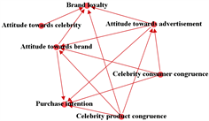
Figure 4. Literature Variables Network.
The pin point direction of the arrowhead of the edges represents the node/ person receiving the message from other nodes/persons and fairly opposite if the node sends the message. For instance, select a node PANNEER from Figure 3; PANNEER is having three pinpoint arrowheads, which means PANNEER is receiving messages from three of his friends KASI, LAVANYA and RIAS. As well as PANNEER sends the message to VENKAT. Map the same SNA concept for literature variable network as shown in Figure 4. In this network the nodes are the variables (independent or dependent) and edges are the connections (directions) between the variables. Since we are dealing with independent and dependent variables in our literature review, independent variables are considered as a “sender” node and dependent variables are considered as “receiver” nodes.
Based on Table 4, literature collation, the digraph is constructed and shown in Figure 4. In Figure 4, the network has 7 nodes and 13 edges in it; 7 nodes are the total number of variables which are used in all the three research papers listed. The 13 edges define the connections between these 7 variables (nodes). Based on the arrowheads we can easily describe whether the variables are an independent or dependent variable. Consider a node, “Attitude towards advertisement”; the total connection (edges) of “Attitude towards advertisement” is five. In these five connections, two arrowheads point towards “Attitude towards advertisement”, which means “Attitude towards advertisement” is a dependent variable (receiving) for two other independent variables/nodes, namely “Celebrity consumer congruence”, and “Celebrity product congruence”. At the same time “Attitude towards advertisement” is acting as an independent variable for other three variables, namely “Attitude towards brand”, “Brand loyalty”, and “Purchase intention”.
Now by embedding the metrics applied to draw insight about an SNA to the literature network, a researcher can quickly summarize the information available among the literature/articles collected and importance of each variable and critical relationship which are often studied or rarely studied to identify a research gap.
5. Metric Result and Discussion
Degree centrality defines the central position of each node (variable) in a network [6] . The position of a node in a network shows the strength of the relationship (edge) between other nodes in the same network. If the number of relationships or immediate contacts of a node is very high in the network, then the particular node is most active with other nodes in the network.
For example, in Figure 5 “Attitude towards advertisement” and “Attitude towards brand” have degree “5”; compared to other variables the value is higher and it shows the importance of these two variables studied with other variables in the literature collection. At the same time, “Attitude towards celebrity” has degree “1” in the network, which is lowest, which signifies that this variable is not much concentrated by previous research works in the literature collection and other variables have moderate degree values. If the direction of the relationship (edges) is important to the network then the degree is classified as in-degree and out-degree centrality.
In-degree centrality measures the number of relationships (edges) received by an ego node (ego variable) from other alters nodes (alters variable). For example, in Figure 6 “Purchase intention” and “Brand loyalty” have very strong receiving relationships (edges) with a degree of “4” compared to other variables in the network. In-degree centrality defines that “Purchase intention” and “Brand loyalty” are the variables studied as dependent variable for more number of times in literature collection. At the same time, “Attitude towards celebrity”, “Celebrity consumer congruence”, and “Celebrity product congruence” are by no means measured as dependent variables by any of the researchers in the literature collection.

Figure 5. Degree Centrality.

Figure 6. In-Degree Centrality.
Out-degree centrality measures the number of relationships (edges) given (sent) by an ego node (ego variable) to other alters nodes (alters variable). For example, in Figure 7 “Celebrity product congruence” has more number of arrows (4 edges) pointing outwards (sending) in the network. This shows that out-degree centrality defines “Celebrity product congruence” is studied more number of times as independent variable in literature collection. Meanwhile, “Brand Loyalty” and “Purchase intension” give values “0”, which means these two variables are measured only as dependent variables in literature collection.
These three measures, viz., degree, in-degree, and out-degree, provides insight to the researchers to understand the positioning of previous research works; significance of a set of variables studied in the past. However these measures do not describe the significant level of other nodes (variables), which are connected to them. Also, these measures do not consider the node’s (variables) influential nature or popularity in literature collection [20] .
Betweenness centrality measures the strength of every node in the network and indicates how often it appears between any two random nodes in the network. The node with higher betweenness score is the more influential in the network, as it acts as a junction for communication between other nodes within the network [6] [21] .
Betweenness centrality differs from degree-centrality in the sense that a node is connected to many other nodes within a cluster (group of nodes) and has few connections to other nodes in other clusters in the network. The node will then be more influential within its cluster provided, it will have less influential connection between other clusters. Thus, Betweenness centrality brings out a node’s interconnections with two or more clusters in the network. In Figure 8, the variables “Attitude towards advertisement” and “Attitude towards brand” have a high betweenness centrality score of “0.5”. This shows that both the variables are acting as a bridge for other variables in the network. At the same time, these two variables are studied as both independent as well as dependent variables in the collected literature.
Betweenness centrality could be useful to throw light on different perspectives of the variables in the literature network; in some cases, the degree centrality of a

Figure 7. Out-Degree Centrality.

Figure 8. Betweenness Centrality.
node will be high but the Betweenness score of that node may be lower; this indicates that the node (variable) is more active within cluster, but less connected with other nodes in different clusters of same network. Identifying these influential nodes (variables) will give more insights on a research problem. Since the network data for this paper are very small, identification of different clusters is more difficult.
A node’s (variable) independency (ability) in the network is measured by Closeness centrality. It means the selected node is not in the central position (degree) in the network, and it relies on others to communicate messages through the network. Thus, the node is close to many other nodes, but it is an independent node. The node (variable) with high closeness centrality has an ability to easily access information in the network. The closeness of a node is measured by shortest distance path between the nodes (variables) in the network. In Figure 9, variables “Attitude towards advertisement”, “Attitude towards brand”, “Celebrity product congruence”, and “Attitude towards celebrity” are relatively close to all other variables in the network and variables, “Brand loyalty” and Purchase intention” are far away from the network. Variables with high closeness centrality value are very independent in the network and have the ability to reach any variables in the network without relying on other variables. In Betweenness Centrality measure, the influential node (variable) is identified; Immediate adjacent [12] [22] [23] [24] of this influential node is another measure of importance in the network, where this is measured by Eigenvector centrality of a node. From Figure 10, the variables, “Purchase intension” and

Figure 9. Closeness Centrality.

Figure 10. Eigenvector Centrality.
“Brand loyalty” have high Eigenvector score “1”. The adjacent variables to “Purchase intension” are “Attitude towards brand―0.256822”, “Attitude towards advertisement―0.042447”, “Celebrity product congruence―0,” and “Celebrity consumer congruence―0”. For “Brand loyalty”, the adjacent variables are “Attitude towards brand―0.256822”, “Attitude towards advertisement―0.042447”, “Celebrity product congruence―0”, and “Attitude towards celebrity―0”.
The variables, “Attitude towards brand” and “Attitude towards advertisement” has already been proved as influential variables in terms of degree and Betweenness centrality. Thus, if any variable has a close tie (connection) with these influential variables, it can dramatically increase the access of other variables in the network. To identify these variables, the Eigenvector centrality is applied for the literature variable data. The Eigenvector centrality resulted that “Purchase intension” and “Brand loyalty” are important variables connected with influencing variables such as “Attitude towards brand (0.2568)” and “Attitude towards advertisement (0.04244)”.
Modularity measures the strength (dense) of division in network module (clusters/groups/communities). It also measures both the density of the links (edges) inside communities and the links (edges) between communities. The community detection mechanism is usually used to detect the modularity [18] [25] [26] in the network. The node (variable) with high density in the network is considered to belong to the same community. For Example, in Figure 11, one can see two different communities of variables; the first community of variables are (green color) “Brand loyalty” and “Attitude towards celebrity”; and the other community of variables are (blue color) “Purchase intension”, “Attitude towards brand, “attitude towards advertisement”, “Celebrity product congruence”, and “Celebrity consumer congruence”. These two communities are further examined by cluster coefficient. Cluster coefficient measures the density of each node (variable) within the community in the network that tends to cluster together. In Figure 12, the variable, “Celebrity consumer congruence” has very high cluster coefficient value of 0.5. This denotes “Celebrity consumer congruence” has a “small world effect” and indicates a greater “cliquishness” in the variable network [19] [27] .
At the same time, the variable, “Attitude towards celebrity” has a cluster coefficient value of 0. It shows the importance of the variable in the network as the variable, “Attitude towards celebrity” is not having any other neighborhood variable to form a cluster. The researchers can easily identify these types of unique variables which are not concentrated in literature collection.
A summary of the result of the literature variable network is given in Table 5. The variables, “Attitude towards advertisement” and “Attitude towards brand” are highly active (degree) in the network. According to literature collection, both the variables are studied (influential) as dependent and independent variables in the literature (Betweenness). In-degree and Eigenvector prove that “Purchase intention” and “Brand Loyalty” are the most measurable (dependence) variables studied by the researches in the literature. “Celebrity product congruence” is measured highly as independent variable and the other variables, “Attitude towards advertisement”, “Attitude towards brand”, and “Attitude towards celebrity” are measured and utilized as most intermediate variables (Closeness) in the literature.

Figure 11. Modularity.
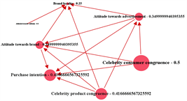
Figure 12. Cluster Coefficient.
Table 5. Overall Results.
Modularity is applied for the overall results (Table 5) and it is shown in Figure 13. The modularity results in three different modules. In module 1 (red color), In-degree and Eigenvector are grouped together with variables, “Purchase intention” and “Brand Loyalty”. These two variables are specifically measured as dependent variables by the research communities. In module 2 (green color), Out-degree and Closeness are grouped together with “Celebrity product congruence”, “Attitude towards celebrity”, “Attitude towards advertisement”, and “Attitude towards brand”. The Out-degree measures the appearance of independent variables in the literature which supports to quantify the significance of dependent variables. Closeness centrality defines the placement of the independent variables in the literature network. Finally, in module 3 (blue color), Degree and Betweenness are grouped with “Attitude towards advertisement” and “Attitude towards brand”. These two variables are more active in the literature and are measured as both independent and dependent variables in literature collection. These are the significant identification and information that can be extracted from the proposed methodology for doing literature review. The proposed methodology gives more insight to the researcher communities to understand the contextual and conceptual flow of research of their specific domain.
6. Conclusions
The research work has made an attempt to develop a framework to analyze the literature collection through Graph Theory metrics. The metrics related to Graph Theory are applied to social network analysis to understand the importance of nodes/persons in the network, clusters of people in the network based on communication among them, and connecting two groups of people; in turn, the current research work correlated these metrics to a literature network and demonstrated a methodology to analyze whether the literature collected is related to a specific research problem. These metrics can easily comprehend volume of data to few numbers. A researcher can develop better insights on careful selection of variables, with a view, whether the variables are frequently studied or less frequently studied: a list of variables to be considered as independent and dependent more scientifically based on centrality measures. A set of variables

Figure 13. Modularity of Overall Results.
can also act as intermediary (moderator/mediator) and relate to some distinct topics of interest.
Measures such as modularity develop deeper insights for the researchers to sense how the variables are grouped and studied in the past. This information may be very difficult to cull out from manual/conventional reviews. However, the researchers are expected to organize the literature into some classification table based on their own convenience to develop such metrics. A word of caution on the list of research papers is considered; the method completely depends upon the quality of input matrix given; the software cannot differentiate a good research work from bad one; or a study which is an original work versus a replication work. Thus, a quality of output usability of the metrics is completely a function of the input matrix developed by the researchers.
7. Limitation and Future Direction
The proposed research work has a few limitations:
Before executing the proposed methodology, the researchers should develop the structured literature data sets. This will be quite time consuming process and also if the researcher is very new to this particular research topic, it will be more complicated to classify the literature data. It needs expert’s opinion about the topic classification.
If the collected literature data does not has a good number of relationships between the documents, the proposed methodology will not be useful for that particular research topic. In general, the researcher should collect literature articles confining to a list of prior defined key words.
The keyword selection should be more appropriate. If the sets of key words are not related, then it will lead to wrong direction and misinterpretation.
The overall modularity results will not be same for every research. It will be different, according to the metrics results.
This paper examined only a small size literature network data.
Future Directions
The researcher should experiment the proposed methodology with a large size data to obtain most significant information from the selected research topics.
In this paper, “Variables literature network” is considered for examination, but the researcher can also consider other literature data such as Objectives and Hypothesis.
This reviewing methodology is applicable for any type of research work with suitable content classification.
Cite this paper
Pachayappan, M. and Venkatesakumar, R. (2018) A Graph Theory Based Systematic Literature Network Analysis. Theoretical Economics Letters, 8, 960-980. https://doi.org/10.4236/tel.2018.85067
References
- 1. Webster, J. and Watson, R.T. (2002) Analyzing the Past to Prepare for the Future: Writing a Literature Review. MIS Quarterly, 26, 13-23.
- 2. Tranfield, D., Denyer, D. and Smart, P. (2003) Towards a Methodology for Developing Evidence-Informed Management Knowledge by Means of Systematic Review. British Journal of Management, 14, 207-222. https://doi.org/10.1111/1467-8551.00375
- 3. Boote, D.N. and Beile, P. (2005) Scholars before Researchers: On the Centrality of the Dissertation Literature Review in Research Preparation. Educational Researcher, 34, 3-15. https://doi.org/10.3102/0013189X034006003
- 4. Petticrew, M. and Roberts, H. (2008) Systematic Reviews in the Social Sciences: A Practical Guide. John Wiley & Sons, Hoboken.
- 5. Rowley, J. and Slack, F. (2004) Conducting a Literature Review. Management Research News, 27, 31-39. https://doi.org/10.1108/01409170410784185
- 6. Freeman, L.C. (1978) Centrality in Social Networks Conceptual Clarification. Social Networks, 1, 215-239. https://doi.org/10.1016/0378-8733(78)90021-7
- 7. Wasserman, S. and Faust, K. (1994) Social Network Analysis: Methods and Applications. Vol. 8, Cambridge University Press, Cambridge. https://doi.org/10.1017/CBO9780511815478
- 8. Butts, C.T. (2008) Social Network Analysis with SNA. Journal of Statistical Software, 24, 1-51. https://doi.org/10.18637/jss.v024.i06
- 9. Everett, M.G. and Borgatti, S.P. (1999) The Centrality of Groups and Classes. The Journal of Mathematical Sociology, 23, 181-201. https://doi.org/10.1080/0022250X.1999.9990219
- 10. Bowers-Campbell, J. (2008) Cyber “Pokes”: Motivational Antidote for Developmental College Readers. Journal of College Reading and Learning, 39, 74-87. https://doi.org/10.1080/10790195.2008.10850313
- 11. Conole, G. and Culver, J. (2010) The Design of Cloudworks: Applying Social Networking Practice to Foster the Exchange of Learning and Teaching Ideas and Designs. Computers & Education, 54, 679-692. https://doi.org/10.1016/j.compedu.2009.09.013
- 12. Venkatesakumar, R. and Pachayappan, M. (2017) Application of Social Network Analysis [SNA] Metrics for Systematic Literature Review [SLR]. Man in India, 97, 233-247.
- 13. Scott, J. (2000) Social Network Analysis: A Handbook. SAGE Publications, Thousand Oaks.
- 14. Bavelas, A. (1950) Communication Patterns in Task-Oriented Groups. The Journal of the Acoustical Society of America, 22, 725-730. https://doi.org/10.1121/1.1906679
- 15. Leavitt, H.J. (1951) Some Effects of Certain Communication Patterns on Group Performance. The Journal of Abnormal and Social Psychology, 46, 38-50. https://doi.org/10.1037/h0057189
- 16. Coleman, J.S. (1973) Mathematics of Collective Action. Transaction Publishers, Piscataway.
- 17. Friedkin, N.E. (1991) Theoretical Foundations for Centrality Measures. American Journal of Sociology, 96, 1478-1504. https://doi.org/10.1086/229694
- 18. Blondel, V.D., Guillaume, J.L., Lambiotte, R. and Lefebvre, E. (2008) Fast Unfolding of Communities in Large Networks. Journal of Statistical Mechanics: Theory and Experiment, 2008, P10008. https://doi.org/10.1088/1742-5468/2008/10/P10008
- 19. Watts, D.J. and Strogatz, S.H. (1998) Collective Dynamics of “Small-World” Networks. Nature, 393, 440-442.
- 20. Kaser, O. and Lemire, D. (2007) Tag-Cloud Drawing: Algorithms for Cloud Visualization.
- 21. Brandes, U. (2001) A Faster Algorithm for Betweenness Centrality. Journal of Mathematical Sociology, 25, 163-177. https://doi.org/10.1080/0022250X.2001.9990249
- 22. Bonacich, P. (1987) Power and Centrality: A Family of Measures. American Journal of Sociology, 92, 1170-1182. https://doi.org/10.1086/228631
- 23. Bonacich, P. (2007) Some Unique Properties of Eigenvector Centrality. Social Networks, 29, 555-564. https://doi.org/10.1016/j.socnet.2007.04.002
- 24. Bonacich, P. and Lloyd, P. (2001) Eigenvector-Like Measures of Centrality for Asymmetric Relations. Social Networks, 23, 191-201. https://doi.org/10.1016/S0378-8733(01)00038-7
- 25. Fortunato, S. (2010) Community Detection in Graphs. Physics Reports, 486, 75-174. https://doi.org/10.1016/j.physrep.2009.11.002
- 26. Ganeshkumar, C., Pachayappan, M. and Madanmohan, G. (2017) Agri-Food Supply Chain Management: Literature Review. Intelligent Information Management, 9, 68-96. https://doi.org/10.4236/iim.2017.92004
- 27. Latapy, M. (2008) Main-Memory Triangle Computations for Very Large (Sparse (Power-Law)) Graphs. Theoretical Computer Science, 407, 458-473. https://doi.org/10.1016/j.tcs.2008.07.017