Abstract

We consider the classical micro-economic foundation of discrete choice, additive random utility models, with conditional utilities depending on expenditure on the numéraire. We show that signs of ownand cross-price effects are identified on the basis of the primal problem only, and Giffen behaviour is ruled out. For the translog specification, we prove that the alternative with highest price behaves as normal good, and the alternative with lowest price behaves as inferior good. We establish conditions for equivalence between the primal and the dual problem. We provide a discrete choice version of the Slutsky equation which, similarly to divisible goods, decomposes the own-price effect into a substitution and an income effect.

Keywords

Discrete Choice, Random Utility, Duality, Price Effects, Income Effects, Slutsky Equation

1. Introduction

Classical consumer theory, which deals with divisible goods, does not restrict how demand changes when price changes, since Giffen goods are not ruled out, or how demand changes when income changes, since both normal and inferior goods are contemplated. Duality provides results that are useful to determine how these two kinds of changes interact.

Duality deals with the relationships between the primal problem, i.e. the utility maximisation under a budget constraint, and the dual problem, i.e. the expenditure minimisation under a utility constraint. Duality is well established. A rigorous treatment is found in micro-economics textbooks by Mas-Colell et al. [1] and Luenberger [2] .

Central to duality is the expenditure function, introduced by McKenzie [3] . It is based on the idea, anticipated by Allen [4] and Hicks [5] , of a compensating behaviour, consisting in an adjustment of income which keeps the consumer, when prices change, on the same indifference locus. Two key results of duality that reveal properties of price and income effects are the primal-dual equivalence and the Slutsky equation.

The equivalence property establishes that: 1) the minimum expenditure, required to achieve the maximum utility achievable with a given income y, is the same income y, and 2) the maximum utility, achievable with the minimum expenditure required to achieve utility level u, is the same utility u. When equivalence holds, the same bundle of goods maximises utility and minimises expenditure, i.e. Marshallian demand equals Hicksian demand.

The Slutsky equation is a consequence of the equivalence property and the Shepard’s lemma. The equation establishes the relationship between the price derivative of the Marshallian demand and the price derivative of the Hicksian demand. Based on this, the marginal effect of a price change is decomposed into a substitution effect, which accounts for the impact at constant utility, and an income effect, which accounts for the impact of the change in real income, the one that occurs when all prices are held constant. The Slutsky equation provides the theoretical justification of the law of demand. This states that the demand response of a normal good to a marginal price increase is negative.

The aim of this note is to extend to discrete choice, the results on price and income effects that in classical consumer theory are provided by duality.

Discrete choice models are usually derived from the assumption of random utility maximisation. A first presentation of the discrete choice, random utility counterpart of classical consumer theory, was provided by McFadden [6] . His approach considers that dependence on economic variables, i.e. prices of the alternatives and income, is through the systematic part of the utilities, and that random terms are independent of observable variables. The latter property defines the class of additive random utility models (ARUMs). All subsequent developments relating to the micro-economic properties of random utility models have been cast within this framework¹. The results in McFadden relate to the primal problem. Among these, there is a qualification of the dependence of systematic utilities on the expenditure on the numéraire as sufficient condition for consistency with Roy’s identity.

Dagsvik and Karlström [7] provided a first treatment of the dual problem for ARUMs. They introduce definitions of the random expenditure function and Hicksian probabilities, together with a treatment of the Shepard’s lemma. Under the usual interpretation of ARUMs that regards the random terms as individual specific, the random expenditure assumes the meaning of an individual-specific expenditure function. The Hicksian probabilities assume the meaning of shares in a population, with homogeneous systematic utilities, where income is being compensated, or, equivalently, expenditure is being minimised, by each individual. Duality in ARUMs has a theoretical interest per se. The extension of duality to a two-period setting, dealt with by Dagsvik and Karlström [7] and Delle Site [8] , is useful for welfare measurement.

To date, price and income effects in ARUMs are still largely unexplored.

The note is organised as follows. Section 2 illustrates the micro-economic foundation of ARUMs, with the formulation of the primal and the dual problem. Section 3 provides properties of price and income effects based on the primal problem. Section 4 establishes the ARUM counterparts of the primal-dual equivalence and the Slutsky equation. Section 5 concludes highlighting commonalities and differences between the divisible good and the discrete choice case.

2. Micro-Economic Foundation

2.1. The Primal Problem

An individual, endowed with income y, consumes a discrete good and a numéraire representing a composite good. The discrete good includes a set of J mutually exclusive alternatives. Given the utility-maximising behaviour subject to a constraint on income spent, when alternative i is chosen the individual will be characterised by a conditional indirect utility function. The utility is expressed by the additively separable structure:, , where is the deterministic component, referred to as systematic utility, and is the random, or error, component. This structure for defines the class of ARUMs.

The systematic utility of each alternative depends on income y, on the price of the alternative, and on other qualitative attributes of the alternative distinct from price. Prices and income are deflated by the price of the numéraire. Taking an additive structure, we have, , where is a function of the qualitative attributes. The function is assumed to be continuous in y and, non decreasing in y and non increasing in.

Therefore, each conditional indirect utility satisfies all the properties to qualify as an indirect utility according to classical consumer theory: continuity in price and income, homogeneity of degree 0 in price and income (since prices and income are deflated), non increasing monotonicity in price, non decreasing monotonicity in income, quasi-convexity in price².

In addition, each conditional indirect utility should generate the demand for the discrete good via Roy’s identity. To achieve this, a sufficient condition is that has a functional form in residual income, i.e. in the expenditure on the numéraire. In the following, we will assume that this property is satisfied. In this case we have:,.

The primal problem (PP) consists in finding the alternative of maximum utility:

(1)

It is easily seen, because of the assumptions made on the conditional indirect utilities, , that the maximum utility U possesses all the properties to qualify as an indirect utility: it is continuous in prices and income, homogenous of degree 0 in prices and income, non increasing in prices and non decreasing in income, quasi-convex in prices. Also, it generates via Roy’s identity the demand for the discrete good:

(2)

The case without income effects, i.e. where income does not affect choice, is obtained when the systematic utilities are linear in residual income with a coefficient that does not depend on alternative, since in this case income cancels out of the maximum function:

(3)

The form commonly used in applied work when income effects are considered is the translog (Herriges and Kling [10] ; Tra [11] ):

(4)

The translog form has the following, desirable, properties. The marginal utility of income depends on the alternative and is inversely related to residual income, being. The intuition is that a dollar has a higher value when the budget available for other expenses is lower. The marginal utility of income decreases with income, which is consistent with the intuition that a dollar provides a decreasing utility as income rises. In addition, if income increases, the difference in utilities of two alternatives with different prices, ceteris paribus, decreases, which means that the difference in market shares decreases too. The intuition is that with higher income the difference in price has a lower impact on demand. Finally, the form ensures that residual income is positive, since so is the argument of a logarithm, a property which is of relevance in the treatment of duality because it implies that compensated income also is positive.

The assumption on the probability distribution of the J-variate random vector defines the ARUM³. Let the random vector be characterized by a probability density function.

In the primal problem, the individual chooses the alternative of maximum utility. The (Marshallian) choice probability is the probability that alternative i is the alternative of maximum utility. Consider the event that alternative i is the alternative of maximum utility:. is a set in the space of the random terms. Therefore:

(5)

where I is the indicator function.

In ARUMs, the derivative of the expectation of the maximum utility U with respect to the systematic utility of one alternative equals the probability of that alternative:

(6)

Williams [13] and Anderson et al. [14] provide a proof of Equation (6) based on differentiation of the expectation of the maximum utility, while Fosgerau et al. [9] provide a proof based on the expression of the expectation of a random variable in terms of its cumulative distribution function.

2.2. The Dual Problem

Given a utility level u, each conditional indirect utility, under the assumptions made, inverts to a conditional expenditure function:, where denotes the inverse of w. The intuition is that, conditional on the choice of alternative i, the individual should compensate income and spend in order to achieve the utility level u.

Each conditional expenditure function satisfies all the properties to qualify as an expenditure function according to classical consumer theory: continuity in price and in the utility level u, homogeneity of degree 1 in price, non decreasing monotonicity in price and in u, concavity in price. In addition, each conditional expenditure function generates the demand for the discrete good via Shepard’s lemma:,.

The dual problem (DP) consists in finding the alternative of minimum expenditure:

(7)

It is easily seen that the minimum expenditure M possesses all the properties to qualify as an expenditure function: it is continuous in prices and in the utility level u, homogeneous of degree 1 in prices, non decreasing in prices and in u, concave in prices⁴. Also, it generates the demand for the discrete good via Shepard’s lemma:

(8)

Notice that, in a random setting, there is no reason why each conditional expenditure function, and hence the minimum expenditure M, should be positive. The individual, depending on her vector of random terms, may need to compensate to an extent to which she runs into debt (i.e. a negative). In the model, this translates into the consumption of a negative amount of the composite good, a circumstance which does not alter the mathematical properties of the quantities of interest (utility and expenditure). However, with a translog specification of the systematic utilities as in Equation (4), we have for any random term vector, because the argument of the logarithm is positive and.

In the dual problem, the individual chooses the alternative of minimum expenditure. The Hicksian, or compensated, probability is the probability that alternative i is the alternative of minimum expenditure with utility u. Consider the event that alternative i is the alternative of minimum expenditure with utility u:. Clearly, this is a set in the J-dimensional Euclidean space of the random terms because each conditional expenditure function, , depends, by definition, on the random term. Therefore, the Hicksian choice probabilities can be expressed in terms of the probability density function of the random terms by:

(9)

3. Results Based on the Primal Problem

The following proposition provides properties of the ownand cross-price effects.

Proposition 1. In ARUMs1) the own-price effects are non-positive:

(10)

2) the cross-price effects are non-negative:

(11)

Proof. First, consider that, in ARUMs, the following hold:

1) the cross-systematic utility derivatives of probabilities are non-positive:

(12)

2) the own-systematic utility derivative of probabilities is non-negative:

(13)

Equation (12) is found in corollary 1 in Fosgerau et al. [9] . The proof is based on the properties that the expectation of the maximum utility exhibits as choice probability generating function.

Since we have, we must have, for a finite change in the systematic utility, and. By taking the limits as approaches 0 we have:

(14)

By combining Equation (12) with Equation (14) we have that, , which is Equation (13).

Since, because of the increasing monotonicity of systematic utility in residual income, we have:

(15)

(16)

Proposition 1 implies that in ARUMs Giffen behaviour is ruled out. The following proposition provides properties of income effects in ARUMs with a translog specification of the systematic utilities.

Proposition 2. In ARUMs with translog specification of the systematic utilities as in Equation (4)1) the alternative with highest price behaves as normal good:

(17)

2) the alternative with lowest price behaves as inferior good:

(18)

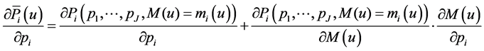
Proof. By the chain rule of derivation (Sydsæter et al. [16] ) we can write:

(19)

Since we are interested in the sign of and, , we can omit the common denominator in Equation (19) and consider the sum:

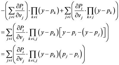
(20)

Since, and, therefore, , Equation (20) can be re-written as:

(21)

Since the Hessian of the expectation of the maximum utility is symmetric and in the light of Equation (6) we have that. Equation (21) can be re-written as:

(22)

Recall that. Therefore, we have that if, , then. If, , then.                                                                              

4. Results Based on Duality

4.1. Primal-Dual Equivalence

The solution of the primal and dual problems is a locus of the random terms, i.e. a set in the J-dimensional Euclidean space, for each alternative. The primal and the dual problems are equivalent when, for each alternative, the locus solution to the problem is the same. Thus, equivalence implies equality of Marshallian and Hicksian probabilities.

The following proposition shows: 1) that the primal problem is equivalent to a dual problem with a properly defined utility level, and 2) that the dual problem is equivalent to a primal problem with a properly defined income level. For clarity of the exposition, we make explicit the income argument of the conditional utilities and of Marshallian probabilities using the notations and. Similarly, we make explicit the utility argument of the conditional expenditure functions using the notation.

Proposition 3. In ARUMs:

1) the primal is equivalent to a dual where the utility level is the maximum utility of the primal:

2) the dual is equivalent to a primal where the income level is the minimum expenditure of the dual:

Proof. For part 1), consider the primal and suppose that i is the alternative of maximum utility:

. Thus,. Then, we have that i is also the alternative of minimum expenditure with utility level equal to U:. This follows from the increasing monotonicity of systematic utilities in residual income (as can be seen simply with the help of a graph in the plane utility-income). Since this holds for any random term vector, we can write for the associated sets of the random terms: , which proves part 1).

The proof of part 2) is similar. Consider the dual and suppose that i is the alternative of minimum expenditure:

. Thus,. Then, we have because of the increasing monotonicity of systematic utilities in residual income. Since this holds for any random term vector, we can write for the associated sets of the random terms:, which proves part 2).          

Proposition 3 establishes an equivalence result at both the individual and the aggregate level. Consider part 1) of the proposition. There are two alternative behavioural models for the individuals. One is the behaviour assumed in the primal problem, with income constraint common to all individuals, where each individual chooses the alternative. The other is the behaviour assumed in the dual problem, with individualspecific utility constraints identified by the choice of the primal problem, where each individual chooses the alternative.

It is proved that each individual makes an identical choice under the two behavioural models, i.e.. At the aggregate level, where the population of individuals is considered, it is proved that an identical sub-population makes choice i under the two behavioural models, i.e.. Notice that the equivalence is established with reference to a dual problem with individual-specific utility constraints. Similar arguments hold for part 2).

Based on proposition 3, we can re-formulate equivalence in the following terms.

Corollary 1. In ARUMs:

1) the minimum expenditure, required to achieve the maximum utility with a given income y, is the same income y:

2) the maximum utility, achievable with the minimum expenditure required to achieve utility level u, is the same utility u:

Proof. For part 1), consider the primal and suppose that i is the alternative of maximum utility:

. Thus,. Then, because of the increasing monotonicity of systematic utilities in residual income, we have that i is also the alternative of minimum expenditure with utility level equal to U:. Therefore we have:, which implies.

For part 2), consider the dual and suppose that i is the alternative of minimum expenditure:.

Thus,. Then, because of the increasing monotonicity of systematic utilities in residual income, we have that i is also the alternative of maximum utility with income level equal to M:. Therefore we have.                                                           

4.2. Slutsky Equation

A consequence of the equivalence property is the ARUM counterpart of the Slutsky equation, which establishes the relationship between the price derivative of the Marshallian probabilities and the price derivative of the Hicksian probabilities.

Proposition 4. In ARUMS1) the own-price derivative of Marshallian probabilities satisfies:

(23)

2) the cross-price derivatives of Marshallian probabilities satisfy:

(24)

Proof. By proposition 3, we can write:, where we have made explicit the price arguments in the Marshallian probabilities. By using the chain rule of derivation (Sydsæter et al. [14] ), derivation with respect to leads to:

(25)

Now consider that we are interested in the conditions where. By corollary 1 we have that the minimum expenditure required to achieve a utility u equal to the maximum utility achievable with income y is the same income y:

(26)

Application of Shepard’s lemma at the individual level yields:

(27)

because.

By substitution of Equations (26) and (27) into Equation (25) we obtain:

(28)

which proves Equation (23) on the own-price effect.

Equation (24) is obtained in a similar way. In this case Shepard’s lemma yields, because the price of alternative j is not an argument of the minimum expenditure.               

Proposition 4 is proved with arguments that are similar to those used to prove Slutsky equation in classical consumer theory. This is because of the equivalence property which is similar in classical theory and ARUMs.

The marginal effect of an own-price change in proposition 4 can be seen as the combination of a substitution effect and an income effect, similarly to classical theory. The intuition is that when the own price changes, we would expect some individuals to shift while the utility achieved is kept the same as before the price change. This is the substitution effect which is captured by the first term in the right-hand side of Equation (23).

With the new price, the expenditure on the alternative changes. The real income changes too and this leads to an additional shift of the individuals who, in so doing, will achieve a new level of utility. This is the income effect which is captured by the second term in the right-hand side of Equation (23).

In the case of a change in the price of another alternative, the intuition is that the income effect is zero because expenditure is unchanged and, therefore, there is no change in real income.

5. Conclusions

The note has extended results on price and income effects to discrete choice.

In the divisible good case of classical consumer theory, price and income effects are considered at the level of the individual consumer. Properties of price effects are revealed by duality theory and the Slutsky equation. Giffen behaviour is possible. The parameter of the dual problem is the utility of the consumer.

In the discrete choice case, under the usual interpretation of ARUMs, price and income effects affect shares, in terms of chosen alternative, of a population of individuals with homogeneous systematic utilities. Properties of price and income effects can be derived on the basis of the primal problem only. Giffen behaviour is ruled out. These results are consequence of the dependence of systematic utilities on the expenditure on the numéraire, a condition which is sufficient to guarantee consistency with the classical micro-economic framework applied to the full set of goods consumed.

Nevertheless, it is possible to establish discrete choice, random utility counterparts of the primal-dual equivalence and the Slutsky equation. The equivalence property and the Slutsky equation are formulated with individual-specific utility parameters in the dual problem. Price responses are decomposed into a substitution and an income effect, but cross-price responses are determined by the substitution effect only.

References

NOTES

¹Recently, Fosgerau et al. have introduced the class of transformed additive random utility models (TARUM), which are of interest because they allow dependence of the random terms on observable variables; the development of an economic theory for this class of models is left for future research.

²A function is quasi-convex on a set C if the sub-level sets are convex, i.e. if for any choice of we have with. A monotonic function of one variable is also quasi-convex (Beer ).

³Random terms are denoted by, specific values by.

⁴The minimum of concave functions is concave (Boyd and Vandenberghe ).

References

- Mas-Colell, A., Whinston, M.D. and Green, J.R. (1995) Microeconomic Theory. Oxford University Press, New York.
- Luenberger, D.G. (1995) Microeconomic Theory. McGraw-Hill, New York.
- McKenzie, L. (1957) Demand Theory without a Utility Index. The Review of Economic Studies, 24, 185-189. http://dx.doi.org/10.2307/2296067
- Allen, R.G.D. (1950) The Substitution Effect in Value Theory. Economic Journal, 60, 675-685. http://dx.doi.org/10.2307/2226707
- Hicks, J.R. (1956) A Revision of Demand Theory. Oxford University Press, Oxford.
- McFadden, D. (1981) Econometric Models of Probabilistic Choice. In: Manski, C. and McFadden, D., Eds., Structural Analysis of Discrete Data with Econometric Applications, MIT Press, Cambridge, 198-272.
- Dagsvik, J.K. and Karlstrom, A. (2005) Compensating Variation and Hicksian Choice Probabilities in Random Utility Models That Are Nonlinear in Income. Review of Economic Studies, 72, 57-76. http://dx.doi.org/10.1111/0034-6527.00324
- Delle Site, P. (2014) On the Expenditure Function and Welfare in Random Utility Models. Economics Bulletin, 34, 152-163.
- Fosgerau, M., McFadden, D. and Bierlaire, M. (2013) Choice Probability Generating Functions. Journal of Choice Modelling, 8, 1-18. http://dx.doi.org/10.1016/j.jocm.2013.05.002
- Herriges, J.A. and Kling, C.L. (1999) Nonlinear Income Effects in Random Utility Models. The Review of Economics and Statistics, 81, 62-72. http://dx.doi.org/10.1162/003465399767923827
- Tra, C.I. (2013) Nonlinear Income Effects in Random Utility Models: Revisiting the Accuracy of the Representative Consumer Approximation. Applied Economics, 45, 55-63.
http://dx.doi.org/10.1080/00036846.2011.589807 - Beer, G. (1993) Topologies on Closed and Closed Convex Sets. Kluwer Academic Publishers, Dordrecht. http://dx.doi.org/10.1007/978-94-015-8149-3
- Williams, H.C.W.L. (1977) On the Formation of Travel Demand Models and Economic Evaluation Measures of User Benefit. Environment and Planning A, 9, 285-344.
http://dx.doi.org/10.1068/a090285 - Anderson, S.P., De Palma, A. and Thisse, J.-F. (1992) Discrete Choice Theory of Product Differentiation. MIT Press, Cambridge.
- Boyd, S. and Vandenberghe, L. (2004) Convex Optimization. Cambridge University Press, Cambridge. http://dx.doi.org/10.1017/CBO9780511804441
- Sydsater, K., Strom, A. and Berck, P. (1998) Economists’ Mathematical Manual. Springer, Berlin.
NOTES
![]()
1Recently, Fosgerau et al. have introduced the class of transformed additive random utility models (TARUM), which are of interest because they allow dependence of the random terms on observable variables; the development of an economic theory for this class of models is left for future research.
2A function  is quasi-convex on a set C if the sub-level sets are convex, i.e. if for any choice of
we have
with
with . A monotonic function of one variable is also quasi-convex (Beer ).
3Random terms are denoted by![]() , specific values by
, specific values by![]() .
.
4The minimum of concave functions is concave (Boyd and Vandenberghe ).