Theoretical Economics Letters
Vol. 2 No. 2 (2012) , Article ID: 19325 , 6 pages DOI:10.4236/tel.2012.22036
Credit, Externalities, and Nonoptimality of the Friedman Rule
1Institute of Economic Research, Hitotsubashi University, Tokyo, Japan
2The Canon Institute for Global Studies, Tokyo, Japan
3Faculty of Economics, Kansai University, Osaka, Japan
4Department of Economics, Senshu University, Kanagawa, Japan
Email: *nutti@isc.senshu-u.ac.jp
Received January 19, 2012; revised March 2, 2012; accepted March 9, 2012
Keywords: Externalities; Cash-Credit Model; Monetary Policy; Friedman Rule
ABSTRACT
We construct a cash-credit model with positive externalities in the production of credit goods. It is shown that under suitable conditions, the Friedman rule is not optimal and there exists an optimal nominal interest rate that maximizes the social welfare and output. This is because increasing the nominal interest rate improves sectoral misallocations caused by externalities in our economy.
1. Introduction
What is optimal monetary policy? A classical answer, provided by Friedman [1], is the Friedman rule—setting the nominal interest rate to zero. As per this rule, a positive nominal interest rate generates inefficiency losses for society since there exists a wedge between the private marginal cost of holding money, which is nominal interest rate, and the social marginal cost of producing money, which is essentially zero. Therefore, it is optimum to set the nominal interest rate to zero. The Friedman rule implies that the central bank should seek a rate of deflation equal to the real interest rate.
In this paper, we construct a two-sector model with cash-goods and credit-goods sectors. It is a cash-credit model developed by Cooley and Hansen [2], Hodrick, Kocherlakota, and Lucas [3], and Lucas and Stokey [4]. An important assumption is that there exist positive externalities in the production of credit goods. We show that under suitable conditions, the Friedman rule is not optimal and there exists an optimal inflation level that maximizes the social welfare and output in our model.
Increasing the nominal interest rate has two effects in our model. The first is a cost, as in standard models. A positive nominal interest rate increases the private opportunity costs of holding money. The second is a benefit. Increasing the nominal interest rate reduces the incentive to hold money and labor input shifts from the cash-goods sector to the credit-goods sector. Since there exist positive externalities in the production of credit goods, this labor input shift has positive effects on the economy. Our results imply that the benefit of increasing the nominal interest rate is greater than the cost if the nominal interest rate is lower than the threshold.
There is extensive literature on the optimality of the Friedman rule.1 For example, Chari, Christiano, and Kehoe [6] find that the Friedman rule is optimal in many frictionless monetary models. Schmitt-Grohè and Uribe [7] show that the optimal nominal interest rate is positive and variable in a sticky-price economy since it acts as a tax on rent. Heer [8] finds that the Friedman rule is not optimal in an economy with search frictions. Bhattacharya, Haslag, and Martin [9], da Costa and Werning [10], and Hiraguchi [11] show that the Friedman rule is not optimal in economies with heterogeneous agents.
This paper is closely related to a paper by Shaw, Chang, and Lai [12] since they show that the Friedman rule is not optimal in a one-sector model with externalities of capital. However, the reason for the non-optimality of the Friedman rule is completely different in both papers. In their model, capital generates production externalities and the capital stock is less than the social optimal level in a competitive equilibrium. Increasing the nominal interest rate encourages the holding of capital and it discourages the holding of money; thus, the social welfare is improved. Contrary to this, in our economy, there exist sectoral misallocations of labor owing to externalities in the production of credit goods. Increasing the nominal interest rate reduces these misallocations of labor and increases the social welfare.
The rest of this paper is organized as follows. Section 2 introduces our model. Section 3 presents our main results: the Friedman rule is not optimal if positive externalities exist in the production of credit goods. Section 4 discusses the reason for externalities and the relationship between taxation and monetary policy in our model. Section 5 concludes the paper.
2. Model
We consider a cash-credit model developed by Cooley and Hansen [2], Hodrick, Kocherlakota, and Lucas [3], and Lucas and Stokey [4]. There is a cash-in-advance constraint for the purchase of cash goods. An important assumption in this paper is that positive externalities exist in the production of credit goods.
2.1. Intermediate Goods Firms
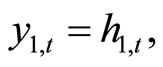
There exist two intermediate goods: cash and credit goods. We assume that both intermediate-goods firms are competitive. The production function of cash-goods firms is
 (1)
(1)
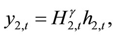
where y1,t denotes cash goods and h1,t denotes labor input for the production of cash goods. For simplicity, we assume that the only factor for the production is labor. The analogue of credit-goods firms is
 (2)
(2)
where y2,t denotes credit goods, H2,t denotes the aggregate labor input of credit goods, and h2,t denotes individual firm’s labor input for the production of credit goods. We assume that γ > 0, that means that positive externalities in the production of credit goods.
2.2. Household
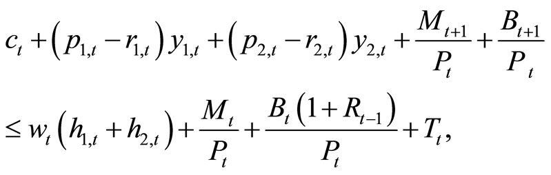
Households supply labor to intermediate-goods firms and earn wages. They buy cash and credit goods from intermediate-goods firms at prices Ptp1,t and Ptp2,t, respecttively, and sell them to final-goods firms at prices Ptr1,t and Ptr2,t, respectively. They buy final goods from final-goods firms ct and possess money Mt and risk-free nominal bonds Bt as assets. The budget constraint of households is
 (3)
(3)
where wt denotes real wage, Rt–1 denotes nominal interest rate, and Tt denotes monetary injection.
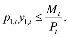
We assume that there is a cash-in-advance constraint for the purchase of cash goods:
 (4)
(4)
Finally, the utility function is
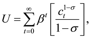 (5)
(5)
where σ > 0 denotes the relative risk aversion and β Î (0, 1) denotes the discount factor of households. In this economy, we assume that total labor supply is constant.
2.3. Case of Elastic Total Labor Supply
Competitive final-goods firms buy intermediate goods from households at prices Ptr1,t and Ptr2,t. They produce and sell final goods to households at price Pt. The production function is constant elasticity of substitution:
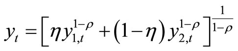 , (6)
, (6)
where 1/ρ>0 denotes the elasticity of substitution between cash and credit goods and η Î (0,1) denotes the share of cash goods in the production of final goods.
2.4. Equilibrium
We consider that the monetary authority sets a nominal interest rate Rt. The market clearing conditions are as follows:
(goods) ,(7)
,(7)
(labor)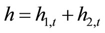 , (8)
, (8)
(bonds) . (9)
. (9)
For simplicity, we consider total labor supply h to be constant.
At the steady state, the equilibrium system is summarized as
 , (10)
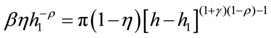 , (11)
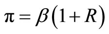
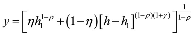 . (12)
Equation (10) shows that the monetary authority controls gross inflation π by setting R. The Friedman rule implies that π = β. Equation (11) is the optimization condition of labor input among two intermediate-goods sectors. Finally, by Equation (12), the output is determined.
3. Nonoptimality of the Friedman Rule
3.1. Main Results
In this paper, we focus on the steady-state relationship between inflation and the social welfare. Since the social welfare depends only on output, we investigate how output is affected by inflation in the following analyses.
Two lemmas are useful for the analyses. The first lemma is on the relationship between output and labor supply in the cash-goods sector.
Lemma 1. The steady-state output y is decreasing in the steady-state labor supply in cash-goods sector h1 if and only if
 . (13)
If , y is increasing in h1.
Proof. Taking total differentiation of (11) yields
 .
.
By the steady-state relationship (12), we obtain
 .
.
A necessary and sufficient condition for  is Equation (13).□
The second lemma is on the relationship between labor supply in the cash-goods sector and inflation.
Lemma 2. The steady-state labor supply in cashgoods sector h1 is decreasing in the steady-state inflation π if and only if
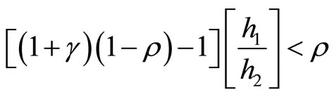 . (14)
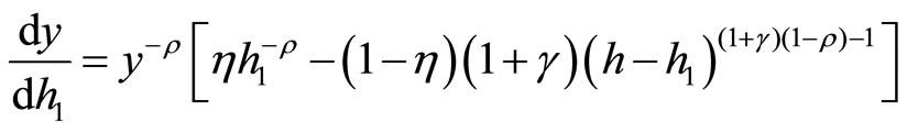
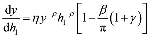
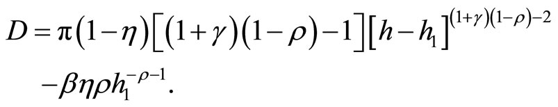
Proof. Taking total differentiation of Equation (12) yields
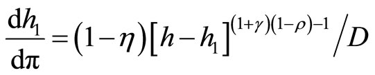 where
where
By the steady-state relationship (12), we obtain
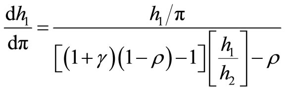 .
.
A necessary and sufficient condition for  is Equation (14).□
Using these two lemmas, we provide two propositions. In the first, no externalities exist: γ = 0.
Proposition 1. If no externalities exist, γ = 0, the Friedman rule is optimal.
Proof. If γ = 0, Equation (14) holds. By Lemmas 1 and 2, it is shown that y is decreasing in π for π ³ β. □
Increasing the nominal interest rate generates inefficiency losses for society since there exists a wedge between the private marginal cost of holding money, which is the nominal interest rate, and the social marginal cost of producing money, which is zero, as in standard models. Therefore, the Friedman rule is optimal in our model without externalities.
If there exist externalities, the optimality of the Friedman rule does not hold under suitable conditions.
The main result in this paper is as follows.
Proposition 2. Assume that γ > 0 and . The Friedman rule is not optimal, and the social welfare is maximized at a steady state with
  and R = γ.
Proof. Since , Equation (14) holds at a steady state with π ³ β. Then, h1 is decreasing in π for all π ³ β. By Lemma 1, it is shown that
  for
for  and
and  for
for . Since the utility function implies that the social welfare is increasing in y, the optimal inflation level is
 . □
. □
In the case with positive externalities in the production of credit goods, increasing the nominal interest rate has positive effects on the economy. By increasing the nominal interest rate, money holding incentive reduces and labor input shifts from the cash-goods sector to the credit-goods sector. Since there exist positive externalities in the production of credit goods, this labor shift has positive effects on the economy. Proposition 2 implies that the benefit of increasing the nominal interest rate is greater than the cost if the nominal interest rate is lower than the threshold.
3.2. Numerical Example
We verify this result by numerical simulations. The model is annual. The discount factor is β = 0.96, which implies that the real interest rate is four percent. The relative risk aversion is σ = 2, following the standard literature. The degree of externalities γ is set such that the optimal inflation is two percent: γ = 0.0625, since the stylized fact shows that economic performance is good under mild inflation rates. We set ρ = 0.065, which satisfies condition (14) and ensures high elasticity of substitution between cash and credit goods. We also set η such that  at a steady state where inflation is two percent: η = 0.5011. In our numerical simulations, the assumption of the interim solution of labor input is satisfied under this value of η.
Figure 1 shows the effect of inflation on steady-state output. We change the steady-state inflation from π = β, that means the case of the Friedman rule, to ten percent. We normalize the output level at π = β to be one hundred. As shown in Proposition 2, output is maximized at a steady state with two percent inflation. The output level at the optimal inflation rate is 1.5 percent higher than that with the Friedman rule. The welfare is also maximized since it is monotone in output in our model.
3.3. Case of Elastic Total Labor Supply
For simplicity, we assume that total labor supply is constant in the model. Here, we relax this assumption. We employ the following utility function:
 , (15)
where σ > 0 and ψ > 0. Other settings are the same as in Section 2.
We investigate the effects of inflation at the steady state by numerical simulations. We set σ so that the

Figure 1. Effects of inflation (1): inelastic total labor supply.

Figure 2. Effects of inflation (2): elastic total labor supply.
steady-state total labor supply is 0.3 and ψ = 2. Other parameter values are the same as in the case of inelastic total labor supply.
Figure 2 shows output, welfare (defined by the utility), and total labor supply given steady-state inflation. We normalize output and total labor level at π = β to be one hundred and welfare to be minus one hundred. In Figure 2, it is shown that even in a model with elastic total labor supply, the Friedman rule is not optimal and there is an optimal inflation level that maximizes the welfare. The optimal inflation is approximately two percent as in the case of inelastic total labor supply. We also find that inflation that maximizes output is less than optimal in this case.
4. Discussions
4.1. Why Do Externalities Exist in the Credit Goods Sector?
Although our assumption that the production of credit goods is associated with positive externalities may seem to be at odds with reality; It might be justified by the network externalities, which are broadly observed in various financial services (King [13]) or privately-issued monetary instruments (Williamson [14]). The credit goods in the present paper are goods that are traded through various financial services, e.g., discounting of promissory notes and payment by credit cards and electronic money. Production of the credit goods in this paper is a reduced-form model of the combined outcome in reality of the goods production and the credit services associated with the trading of the goods. The financial services exhibit network externalities in general (see, for example, Van Hove [15]). This is because various financial services have the nature of network goods, the per-capita cost of which decreases as the number of participants into the network increases. Therefore, our assumption that there exist positive externalities in the production of credit goods can be justified as a shortcut to formalize the network externalities involved in financial services.
We should argue for the plausibility of the degree of externalities in our numerical example. We set γ = 0.0625 to have the optimal inflation at two percent. Harrison [16] shows that there exist externalities in the production of investment goods, the degree of which is within the range of 0.07 or greater. Since the investment goods in Harrison’s estimation and the credit goods in our model seem to overlap to a large extent, her results may be interpreted as supportive of our requirement that γ should be 0.06 or greater for mild inflation to be optimal.
4.2. Taxations and Monetary Policy
In our model, we assume that there exist no fiscal policy and taxes. This might be a strong assumption. Recent studies find that the optimality of the Friedman rule is closely related to the flexibility of the government’s fiscal policy. Correia, Nicolini, and Teles [17] find that if the fiscal policy is sufficient flexible, the Friedman rule is optimal even in a sticky-price economy while SchmittGrohè and Uribe [7] show that the optimal interest rate is positive under an inflexible government fiscal policy.
If the government could levy different taxes on the profits of cash-goods and credit-goods firms, the Friedman rule would be optimal in our economy. In our economy, increasing the nominal interest rate improves the sectoral misallocations of labor caused by externalities, resulting in the non-optimality of the Friedman rule arises. Sectoral tax rates can also improve these misallocations of labor and there are no welfare costs of inflation in this case.
However, it is difficult to distinguish between cash and credit goods in the real world. For example, goods would be categorized as cash goods when they are bought for cash and credit goods when bought using a credit card. Therefore, we believe that our assumption of inflexible fiscal policy is reasonable.
5. Concluding Remarks
In this paper, we construct a cash-credit model with positive externalities in the production of credit goods. Under suitable conditions, the Friedman rule is not optimal and there is an optimal inflation level that maximizes the social welfare in our model, since increasing the nominal interest rate shifts the labor input from the cash-goods sector to the credit-goods sector.
6. Acknowledgements
We would like to thank R. Anton Braun, Ryoji Hiraguchi, Kaoru Hosono, Tsutomu Watanabe, Hiroshi Yoshikawa, and the seminar participants at the Canon Institute for Global Studies for their helpful comments and discussions. All remaining errors are our own. The views expressed in this paper are those of the authors and do not necessarily reflect the official views of any affiliations of the authors.
REFERENCES
- M. Friedman, “The Optimum Quantity of Money,” The Optimum Quantity of Money and Other Essays, Macmillan, London, 1996.
- T. F. Cooley and G. D. Hansen, “Welfare Costs of Moderate Inflation,” Journal of Money, Credit and Banking, Vol. 23, No. 3, 1991, pp. 483-503.
- R. J. Hodrick, N. Kocherlakota and D. Lucas, “The Variability of Velocity in Cash-in-Advance Models,” Journal of Political Economy, Vol. 99, No. 2, 1991, pp. 358-384.
- R. E. Lucas and N. L. Stokey, “Money and Interest in Cash-in-Advance Economy,” Econometrica, Vol. 55, No. 3, 1987, pp. 491-513. doi:10.2307/1913597
- M. Golosov and A. Tsyvinski, “Optimal Fiscal and Monetary Policy (with Commitment),” In: S. N. Durlauf, L. Blume, Eds., Monetary Economics (The New Palgrave Economic Collections), 2010, pp. 277-282.
- V. V. Chari, L. Christiano and P. Kehoe, “Optimality of the Friedman Rule in Economies with Distorting Taxes,” Journal of Monetary Economics, Vol. 37, No. 2-3, 1996, pp. 203-223. doi:10.1016/S0304-3932(96)90034-3
- S. Schmitt-Grohè and M. Uribe, “Optimal Fiscal and Monetary Policy under Sticky Prices,” Journal of Economic Theory, Vol. 114, No. 2, 2004, pp. 183-209. doi:10.1016/S0022-0531(03)00111-x
- B. Heer, “Welfare Costs of Inflation in a Dynamic Economy with Search Unemployment,” Journal of Economic Dynamics and Control, Vol. 28, No. 2, 2003, pp. 255-272. doi:10.1016/S0165-1889(02)00136-7
- J. Bhattacharya, J. Haslag and A. Martin, “Heterogeneity, Redistribution, and the Friedman Rule,” International Economic Review, Vol. 46, No. 2, 2005, pp. 437-454. doi:10.1111/j.1468-2354.2005.00327.x
- C. da Costa and I. Werning, “On the Optimality of the Friedman Rule with Heterogeneous Agents and Non- Linear Income Taxation,” Journal of Political Economy, Vol. 116, No. 1, 2008, pp. 82-112. doi:10.1086/529397
- R. Hiraguchi, “Wealth Inequality and Optimal Monetary Policy,” Macroeconomic Dynamics, Vol. 14, No. 5, 2010, pp. 629-644. doi:10.1017/S1365100509990885
- M. Shaw, J. Chang and C. Lai, “(Non)Optimality of the Friedman Rule and Optimal Taxation in a Growing Economy with Imperfect Competition,” Economics Letters, Vol. 90, No. 3, 2006, pp. 412-420. doi:10.1016/j.econlet.2005.10.002
- M. King, “The Institutions of Monetary Policy,” American Economic Review, Vol. 94, No. 2, 2004, pp. 1-13. doi:10.1257/0002828041301957
- S. D. Williamson, “Private Money,” Journal of Money, Credit and Banking, Vol. 31, 1999, pp. 469-491.
- L. Van Hove, “Electronic Money and the Network Externalities Theory: Lessons for Real Life,” Netnomics, Vol. 1, No. 2, 1999, pp. 137-171. doi:10.1023/A:1019105906374
- S. G. Harrison, “Returns to Scale and Externalities in the Consumption and Investment Sectors,” Review of Economic Dynamics, Vol. 6, No. 4, 2003, pp. 963-976. doi:10.1016/S1094-2025(03)00034-6
- I. Correia, J. P. Nicolini and P. Teles, “Optimal Fiscal and Monetary Policy: Equivalence Results,” Journal of Political Economy, Vol. 116, No. 1, 2008, pp. 141-170. doi:10.1086/533504
Appendix
The equilibrium system of our economy is as follows.
 ,
,
 ,
,
 ,
,
 ,
,
 ,
,
 ,
,
 ,
,
 ,
,
 ,
,
 ,
,
 where
where  denotes gross inflation,
 denotes real money balances, and μt denotes the ratio of the Lagrange multiplier of the cashin-advance constraint to that of the budget constraint.
NOTES
*Corresponding author.
1See a review by Golosov and Tsyvinski [5] for details on this literature.