Journal of Mathematical Finance
Vol.06 No.01(2016), Article ID:63958,12 pages
10.4236/jmf.2016.61016
Statistical Arbitrage in S&P500
Stefanos Drakos
International Centre for Computational Engineering, Rhodes, Greece
![]()
Copyright © 2016 by author and Scientific Research Publishing Inc.
This work is licensed under the Creative Commons Attribution International License (CC BY).
http://creativecommons.org/licenses/by/4.0/


Received 8 January 2016; accepted 24 February 2016; published 29 February 2016
ABSTRACT
A methodology to create statistical arbitrage in stock Index S&P500 is presented. A synthetic asset based on the cointegration relationship of the stocks with Index was constructed. In order to capture the dynamic of the market time adaptive algorithms have been developed and discussed. The pair trading strategy was applied in different periods between S&P500 and synthetic asset and the results were evaluated. Different metrics have shown that the Multvariate Kalman Algorithm creates statistical arbitrage in index with much lower Maximum Drawdown and higher profit. The algorithm is neutral as the beta is close to zero and the Sharp Ratio remains high in all cases.
Keywords:
Statistical Arbitrage, Mean Reverting, Pair Trading, Kalman Filter, Trading Algorithms

1. Introduction
Financial markets are based on the general trading rule: buy with low price and sell with high price. The aim is the development of strategies with low risk and succeeds this general rule. Pure Arbitrage is a category of strategies with zero risk. As an example we can refer the case of buying and selling a stock at the same time with a different value in two different exchanges. The profit results from the difference in prices, breaking the law of one price.
Another category is the statistical arbitrage which is not risk free at all. Strategies of this type are aimed at the expected gain which is greater than the risk. The profit results from the mispricing of the stocks. To achieve this, one needs to assess whether the price of a stock is overvalued or undervalued relative to the actual value which is really hard to determine. The fundamentals of the stock, the demand of each period and the general economic environment are some of the factors that make the fair value evaluation difficult. Part of this category is the Pair Trading and is presented in several references as in [1] -[10] . The Pairs trading is a strategy which is based on the relative pricing of stocks without actually interested in the true value of them. The relative pricing is based on the idea that two assets with the same features can be priced about the same price as the basis of the law of one price. When at a given time the stock prices are different then one is overvalued and the other undervalued relative to the actual price. The classic trading Pairs strategy derives from the characteristics of this incorrect pricing (mispricing) between the two stocks.
In the current work instead of the two stocks the mispricing between the index S&P500 and a sub-set of stocks belonging to this is considered. This forms a portfolio consisting of one unit of the Index in long (or short) and the corresponding number γ (Hedge ratio) of subset’s stocks in the opposite position. Three methods adopted to determine the number γ (Hedge ratio): a) the ordinary, b) the rolling ordinary least squares (OLS) regression and c) the Kalman filter process as it is presented below. According to the strategy, the spread of the index S&P500 and the stocks prices’ combination are computed and when this deviates from its historical average value then the investor bets on the return to the historical with selling and buying respectively the stocks of the portfolio. In practice to construct the synthetic asset is necessary to investigate the appropriate stock exhibiting long relationship between them with the index. The technique used for this purpose is the Cointegration as this presented in [1] according to which two time series  and
and  are cointegrated if
  for
for  and notation I(d) means integrated order d.
In [1] concluded that pairs who cointegrate in sample period behave better in the out-of-sample period than those not cointegrate in the sample period. Based on the previous, the spread of the linear combination of the cointegrated stocks and the S&P500 index have to be stationary process. To analyze this relationship the augmented Dickey-Fuller test (ADF) was used as presented in [2] . According to the strategy the stocks are not restricted to cointegrate in the out-of-sample period but it is an indication that they will present mean-reverting behavior.
Additionally the log of prices used is also instead the prices as in [3] . The main reason is that log-returns are time additive. So, in order to calculate the return over n periods using real returns we need to calculate the product of n numbers:![]() .
.
If ![]() defined as:
defined as:
![]() (1)
(1)
And
![]() (2)
(2)
![]()
Consequently the profit of spread over a period is equal to:
![]() (3)
(3)
The classic application of the trading pair strategy has published in many works in the past and has been applied in practice. In [4] the author went a further step and presented an algorithm for the pair trading of a stock basket cointegrated with the S&P500 using constant cointegrating coefficient with a single value for all stocks belonging to the basket. To capture the real behavior of the markets this work presents new Time Adaptive algorithms using rolling ordinary least squares (OLS) regression and Multivariate Kalman Filter process where the time dependent hedge ratio is computed separately for each of the stocks forming the synthetic asset creating thereby statistical arbitrage conditions in index S&P500 and increasing the strategy performance.
2. Period of Methodology
The proposed methodology and the trading algorithm designed based on that divided in two different spaces. The first refers to the in sample period which is used to make all the appropriate test and construct the synthetic asset and the other to the out of sample period (Trading Period) where the synthetic asset trading based on the specific rules (Figure 1).
2.1. In Sample Period
The data of the in sample period used for the synthetic asset construction. Working on a daily data domain a year of closing prices was chosen as the in sample period for determine the set of cointegrated stocks with S&P500 and create the synthetic asset.
Synthetic Asset Construction.
The paper presents different algorithms in order to create statistical arbitrage in S&P500. The S&P500, based on themarket capitalizations of 500 large companies equity indices, and many consider it one of the best representations of the U.S. stock market. The initial choice of stocks for cointegration test with S&P500 is made by the S&P100 which is a sub-set of the S&P500, and measures the performance of large cap companies in the United States. Constituents of the S&P100 are selected for sector balance and represent about 57% of the market capitalization of the S&P500 and almost 45% of the market capitalization of the U.S. equity markets. The stocks in the S&P100 tend to be the largest and most established companies in the S&P500 (Wikipedia).
Using the data of a selected In Sample Period for each stock ![]() the second step of Engle and Granger’ approach adopted. Using the logarithmic price of stocks and S&P500 the OLS regression shown below is performed:
the second step of Engle and Granger’ approach adopted. Using the logarithmic price of stocks and S&P500 the OLS regression shown below is performed:
![]() (4)
(4)
Τhe Augmented Dickey-Fuller unit root test applied for the stationarity of the OLS residuals. According to the successful stationary result a subset of the S&P100 is created and the components of this set are the candidate for the synthetic asset construction. Still working in the sample period a new OLS regression was carried out:
![]() (5)
(5)
Or
![]() (6)
(6)
Using again the Augmented Dickey-Fuller the stationarity of the new OLS residuals is examined.
If the stationarity exist then this an evidence of mean reverting long term behavior of the spread
 where
where  and S is the set of stock where individually and as logarithmic
sum cointegrated with S&P500. The dimension of S is dim(S).
2.2. Out of Sample Period-Trading Period
According to the previous period different algorithms for synthetic asset trading are developed. The first was

Figure 1. Period of study.
designed assumed that the cointegration coefficient is constant during the trading period.
In that case and using the Equation (3) the profit of the strategy during the period t ÷ t + h arises from the following equation:
 (7)
(7)
3. Time Adaptive Coefficient γ
In reality the system of trading is dynamic and updated as new information get to in and the cointegration coefecient (or the hedge ratio) cannot stay constant during the trading period. For that reason time adaptive algorithms are developed to capture the real conditions of the markets.
3.1. Rolling Ordinary Least Squares (OLS) Regression
The first one considering a rolling ordinary least squares (OLS) regression. The frequency of regression calculations raised by an optimization procedure and the cointegration coefficient calculated at each step by the regres-
sion of  against the
 .
.
3.2. Kalman Filter Process
The Kalman filter process can be described by three different steps: the prediction the observation and the correction. A new approach were developed using a Multivariate Kalman filter process. Based on that the hedge ratio calculated separately for each stock owned in the synthetic asset and the computed vector of the calculated parameters at each time step has dimensions (N + 1) × 1 where N = dim(S) while the dimensions of the covariance matrix is (N + 1) × (N + 1). The aim of these algorithms is to calculate at each time step the updated hedge ratio of the synthetic asset. Assuming that the hedge ratio and the premium follow a random walk we have:
 (8)
(8)
where:
yt: is the current state of the of the parameters.
yt-1: is the previous state of the of the parameters.

where for the multivariate Kalman filter process
 (9)
(9)
With:
 (10)
(10)
h: is the cointegration coefficient from in sample period and μ0 coming from the same period.
The vector of logarithmic price of stocks:
 (11)
(11)
And 
The process following the steps as below:
Prediction state where the next system state is predicted based on the knowledge of the previous state
 (12)
(12)
The covariance of prediction state is given by:
 (13)
(13)
The next step concerns the measurement prediction. Given the price of the synthetic asset and the predicted hedge ratio the measurement prediction are given as:
 (14)
(14)
The residual of measurement and real value at each step calculated as:
 (15)
(15)
The variance of measurement error is equal to:
 (16)
(16)
The Kalman Gain is the filter, which tells how much the predictions should be corrected on time step is given as:
 (17)
(17)
The last step of process is the update step where:
The updated state is estimated as following:
 (18)
(18)
And the Updated state covariance is equal to
 (19)
(19)
All the process repeated at every time step of out of sample period. The estimation of Vw and Ve has been discussed in [11] [12] .
3.3. Profit of Strategies
In the case of Time Adaptive coefficient γ of the linear regression case the profit of the pair trading strategy raised by the following equations:
 (20)
(20)
In the case of Multivariate Kalman Filter where the hedge ratio is different for each stock and for each time step in the synthetic asset it can been shown that:

Similarly

And finally the profit during a period  is equal to:
 (21)
(21)
4. The Pair Trading Strategy
The algorithm of the pair trading strategy is based on the distance of the spread from its historical mean value and its mean-reverting behavior. To measure this distance a normalized variable called z-score introduced as:
 (22)
(22)
where:
 : is the mean value of the spread over a lookback period.
 : is the standard deviation of the spread over the same period.
The trading it takes place when this variable exceeds some limits based on the spread mean reverting behavior. Thus:
Open-long position if .
.
Open-short position if .
.
Exit-long position if .
.
Exit-short position if .
.
When a long (short) position is opened we buy (sell) one unit of S&P500 and sell (buy) the following amount
of stocks from synthetic asset as:  in the case of constant hedge ratio,
  when the rolling OLS regression is applied, and
  if the Kalman Filter algorithm applied. The performance
of strategy evaluated using the following metrics: 1) Cumulative return, 2) Annualized Return, 3) Sharpe Ratio, 4) Maximum drawdown, 5) beta.
5. Back Testing-Performance Evaluation
Five different time periods was studied. In each case one year data collection was used in order to make the entire test and construct the synthetic asset. After that the algorithm starts trading with ending day for all cases the 30/12/2015. All the sample periods started at the first day of the year and ending at the last of the same year. The trading started on the first day the next year. In Table 1 the back testing periods are presented. In Figure 2 and Figure 3 the results of cumulative return of Multivariate Kalman Filter algorithm against S&P500 and its maximum drawdown are shown. In Figure 4 and Figure 5 the cumulative return of rolling OLS regression algorithm against S&P500 and the cumulative return of rolling OLS regression algorithm against constant hedge ratio are illustrated. In t Table 2 the sets of synthetic assets are presented while in Table 3 the name of symbols is given. In Tables 4-8 all the metrics of the algorithms are displayed.
It can be shown that the dimension of the set and the constituents are different from period to period. This is an evidence of the non constant cointegration behavior of the stocks with the index but as we can see from the graphs the synthetic asset of each period continues to trade with profit and good metrics results.

Table 1. Back testing periods.
Table 2. Sets of stock in synthetic asset on each period.
Table 3. Union set of companies raised from cointegration test from all the period of study.
Table 4. Statistical metrics performance for the trading period 01/01/2007-30/12/2015.
Table 5. Statistical metrics performance for the trading period 01/01/2008-30/12/2015
Table 6. Statistical metrics performance for the trading period 01/01/2010-30/12/2015
Table 7. Statistical metrics performance for the trading period 01/01/2010-30/12/2015
Table 8. Statistical metrics performance for the trading period 01/01/2011-30/12/2015

Figure 2. Cumulative return and drawdown diagram for multivariate kalman filter algorithm for the trading periods starting at 2007, 2008 and ending at 2015.
Comparing the metrics of each period of study it is clear the Multivariate Kalman Filter algorithm gives the better results among the other and the Index S&P500. In the first period where the Index presents the higher Maximum Drawdown equal to 62% and cumulative returns (CR) equal to 45.59% (Annualized percentage APR = 4.26%) the Multivariate Kalman filter algorithm (MKFA) gives the highest cumulative rate result = 387% (with APR = 19.26%) with a reasonable Maximum Drawdown (MDD) = 12.64 and duration = 73 days. The MKFA in other cases shows max CR = 278% (APR = 20.9%) and Sharpe Ratio = 3.039 while in trading period 2008-2015 present the higher MDD = 28.63 with duration = 175 days. At the same period the Index presents MDD = 52.9% with duration = 154 days. The profit from MKFA given by CR = 172% (APR = 13.32) and on the other hand S&P500 has CR = 42.47% (APR = 4.52%). In this period the MKFA has the lowest SR = 1.13 but still higher than Index. The lower CR of MKFA given in the period 2011-2015 and equal to 81.34% (APR = 12.67%) with MDD = 8.51% and duration = 125 days. In this trading period the index has CR = 62% (APR = 10.16%) but
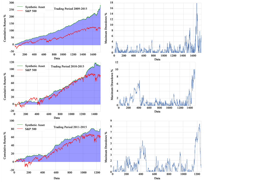
Figure 3. Cumulative return and drawdown diagram for multivariate kalman filter algorithm for the trading periods starting at 2009, 2010, 2011 and ending at 2015.

Figure 4. Cumulative return of rolling ols regression algorithm against S&P500 and algorithm with constant hedge ratio, for trading period starting AT 2007, 2008, 2009 and ending at 2015.

Figure 5. Cumulative return of rolling OLS regression algorithm against S&P500 and algorithm with constant hedge ratio, for trading period starting at 2010, 2011 and ending at 2015.
with higher MDD = 23.42 and duration = 203. The SR of MKFA is still higher and equal to 2.313. In the last periods the profits declined but kept higher profit and Sharp Ratio than S&P500.
The second algorithm of rolling OLS regression gives lower cumulative profit than Index but has almost doubled Sharp Ratio than S&P500 in all cases. Finally the evaluation of metrics has shown that the MKFA can beat the market as it creates statistical arbitrage condition in Index.
6. Conclusion
Mean-reverting algorithms with time adaptive hedge ratio are presented. A methodology of a synthetic asset construction based on the stocks of S&P500 has been discussed. The criterion of the selection was the cointegration relationship of individual stocks as the logarithmic sum of them with S&P500. The results of back testing show that for different period of study the form and the dimension of the synthetic asset are different. Pair trading strategy was adopted and the evaluation of the metrics results presented better behavior of MKFA among the others and beat the market. In the last periods the profits declined but it was still higher than S&P500 with much higher Sharp Ratio. The algorithm defended better its profit as the Maximum Draw down was quite lower than Index.
Cite this paper
StefanosDrakos, (2016) Statistical Arbitrage in S&P500. Journal of Mathematical Finance,06,166-177. doi: 10.4236/jmf.2016.61016
References
- 1. Engle, R. and Granger, C. (1987) Co-Integration and Error Correction: Representation, Estimation, and Testing. Econometrica, 55, 251-276.
http://dx.doi.org/10.2307/1913236 - 2. Vidyamurthy, G. (2004) Pairs Trading, Quantitative Methods and Analysis. John Wiley & Sons, Hoboken.
- 3. Infantino, L. and Itzhaki, S. (2010) Developing High-Frequency Equities Trading Models. Master of Business Administration, Massachusetts Institute of Technology, Cambridge.
- 4. Ernie, C. (2013) Algorithmic Trading: Winning Strategies and Their Rationale. John Wiley & Sons, Hoboken.
- 5. Caldeira, J. and Moura, G.V. (2013) Selection of a Portfolio of Pairs Based on Cointegration: A Statistical Arbitrage Strategy.
http://dx.doi.org/10.2139/ssrn.2196391 - 6. Dunis, C.L. and Ho, R. (2005) Cointegration Portfolios of European Equities for Index Tracking and Market Neutral Strategies. Journal of Asset Management, 6, 33-52.
http://dx.doi.org/10.1057/palgrave.jam.2240164 - 7. Dunis, C.L, Giorgioni, G., Laws, J. and Rudy, J. (2010) Statistical Arbitrage and High-Frequency Data with an Application to Eurostoxx 50 Equities. CIBEF Working Papers, CIBEF.
- 8. Elliott, R., van der Hoek, J. and Malcolm, W. (2005) Pairs Trading. Quantitative Finance, 5, 271-276.
http://dx.doi.org/10.1080/14697680500149370 - 9. Gatev, E., Goetzmann, W.N. and Rouwenhorst, K.G. (2006) Pairs Trading: Performance of a Relative-Value Arbitrage Rule. Review of Financial Studies, 19, 797-827.
http://dx.doi.org/10.1093/rfs/hhj020 - 10. Khandani, A. and Lo, A.W. (2007) What Happened to the Quants in August 2007.
http://web.mit.edu/Alo/www/Papers/august07.pdf - 11. Rajamani, M. (2007) Data-Based Techniques to Improve State Estimation in Model Predictive Control. PhD Thesis, University of Wisconsin-Madison, Madison.
- 12. Rajamani, M.R. and Rawlings, J.B. (2009) Estimation of the Disturbance Structure from Data Using Semidefinite Programming and Optimal Weighting. Automatica, 45, 142-148.
http://dx.doi.org/10.1016/j.automatica.2008.05.032