Wireless Sensor Network, 2010, 2, 318-327
doi:10.4236/wsn.2010.24043 Published Online April 2010 (http://www.SciRP.org/journal/wsn)
The Optimal Sensing Coverage for Road Surveillance
X. F. Cheng, P. Liu, Z. G. Chen, H. B. Wu, X. H. Fan
New Star Research institute of Applied Technology, Hefei, China
Received January 15, 2010; revised February 20, 2010; accepted March 4, 2010
Abstract
So far path coverage problem has been studied widely to characterize the properties of the coverage of a path
or a track in an area induced by a sensor network, in which the path or track is usually treated as a curve and
the width of it can be ignored. However, sensor networks often are employed to carry out road surveillance
or target tracking, in which the interesting area is only the surface of the road, thus the width of the road must
be considered. This paper analyzes the optimal sensing coverage of the road in this kind of applications, as-
suming that sensor nodes are deployed along both sides of the road determinately. The optimal position of
sensor nodes is studied considering the sensing range of sensors and the width of the road, and the purpose is
to cover the road surface completely with minimal nodes. The isosceles triangle model is proposed and
proved to be the most suitable, that is to say all sensors get the maximal available sensing area if any three
nearest sensors located on both sides of the road form an isosceles triangle. Comparing with the equilateral
triangle model proposed in other articles, this model increases the coverage rate and supplies complete cov-
erage of the road.
Keywords: Sensor, Network, Optimal, Coverage, Road
1. Introduction
Coverage is an important performance index of a sensor
network, because it represents how well the object of
interest is monitored by sensors, or how effective a sen-
sor network is in detecting objects intruding the field of
watch. Knowing the fundamental coverage property of a
sensor network helps to better construct sensor networks.
For example, it could tell us how densely sensors should
be deployed to detect an intruding object with a given
probability or to trace a given fraction of trajectory of the
object.
Road surveillance is an important kind of applications,
and can be used for traffic surveillance, overspeed early
warning, target detection and classification etc. Unat-
tended road surveillance can be realized by wireless
sensor network, which is quite economical of manpower
and the efficiency of surveillance is also improved, and it
is a new direction for application research of wireless
sensor network [1,2].
The aim of this work is to analyze the coverage prop-
erty of a sensor network, which is deployed determi-
nately along both sides of a road. In particular, we focus
on the optimal sensing coverage, in order to get complete
coverage over the road and connectivity between sensors,
using minimal number of sensors. It is fundamental in
some applications, such as road surveillance, target trac-
ing and others. Because it not only determines the cost of
a network, but also influences the veracity and validity of
the results. In those applications, the width of the road
and the sensing range of sensors must be taken into ac-
count, because they are primary factors which affect the
relative position among deployed sensors.
The path coverage problem has been extensively stud-
ied in recent years, which is useful for the study of this
paper. For example, Junko Harada et al. [3] analyzed the
path coverage property of a sensor network, character-
ized the path coverage in terms of three metrics: fraction
of coverage, probability of complete coverage, and
probability of partial coverage, and derived the expres-
sions for the three coverage metrics as functions of the
sensor density, the sensing range of a sensor, and the
communication range of a sensor. Pallavi Manohar et al.
[4] analyzed the statistical properties of the coverage of a
one-dimensional path induced by a two dimensional non
homogeneous random sensor network. Sundhar Ram et
al. [5] analyzed the one-dimensional path-coverage in-
duced by an area coverage process in a random sensor
network and obtain the trackability measures defined in
the literature. k-track coverage [6] investigated the prob-

X. F. CHENG ET AL.319
lem of finding the configuration of a network with n
sensors so that the number of tracks intercepted by k
sensors is optimized without providing redundant area
coverage over the entire region. These studies considered
the coverage property of a path or a track in an area in-
duced by a sensor network. Expressions or formulas de-
rived in these papers are not suitable for the problem
proposed in this paper.
Kurlin et al. [7] proposed a method to find the mini-
mal number of sensors randomly deployed along a
one-dimensional path to make a network connected with
a given probability. The paper also described a powerful
method for explicitly computing the probability of con-
nectivity of 1-dimensional networks. However, the path
coverage probability is not taken into account, which is
vital in road surveillance applications.
The optimal configuration of sensor nodes has also
been focused on, such as the equilateral triangle model
[8], which means that if the region R is large enough as
compared to the sensing range of each sensor node, to
cover region R completely with minimal number of
nodes, sensor nodes should be placed as follow: any
three disks composed by the coverage area of a sensor
node centered at itself should intersect at one point and
form an equilateral triangle with side length3
s
r, where
is the sensing range of sensors, see Figure 1. Since
sensor nodes can but be placed along both sides of the
road in the kind of road surveillance application, they
form an equilateral triangle if and only if the width of the
road d objects to (1). However, the width of the road may
vary from a couple of meters to dozens of meters, and
the sensing range of sensors is also variable in practice,
and both of them can not object to (1) in most times.
s
r
3
3sin
32
s
s
dr

 r (1)
The contribution of this work is to analyze the optimal
sensing coverage for road surveillance taking account of
the sensing range of sensors and the width of the road. As
a result, we find that the maximal available sensing area of
the networked sensors can be achieved when the positions
of every three closest sensors form an isosceles triangle.
The rest of this article is organized as follows. In Section 2,
s
r
s
r3
Figure 1. The equilateral triangle model.
we present some related background on the road cover-
age. In Section 3, we analyze the optimal sensing cover-
age, present and prove our propositions while the sensing
d d subject to range of sensorssand the width of the roa
/2 s drd
r

and s rd respectively. In Section 4, we
the conclusion of this paper.
. Background of Road Coverage
Ro
compare our isosceles model with the equilateral model.
Some simulation experiments about the number of sensor
nodes required to cover a road optimally have been done
based on our research results in Section 5. The Section 6
is
2
ad surveillance and target tracking are common appli-
cations of Wireless Sensor Network. The coverage prob-
ability varies from different purpose, and we assume that
we need to cover the road surface completely in this paper.
2.1. Sensing Model
We assume that each sensor has the same sensing range,
s
r. A sensor can detect all events within isensin
range with probability 1, but it cannot detect any events
at all outside the sensing range. This simplified sensing
model is usually called “Boolean sensing model” [9,10].
We also assume that each sensor has an identical
communication range, rw. A sensor can communicate
with all sensors within its communication range.
Zhang et al. [8] proved that the conditi
ts g
on of ≥ 2
ensure that complete
overage of a convex region implies connectivity in an
and the road surface in
practice. Thus they are usually placed along both sides of
e
sens the road.
2.3. Relaad and
Sensing Range of Sensors
d and sensing range of sensors
w
r s r
is both necessary and sufficient to
c
arbitrary network, assuming the monitored region is a
convex set. For clarity of discussion, we assume that
communication range is at least twice of sensing range in
this paper, and then the set of sensor nodes is connective
if it covers the road surface completely.
2.2. Structure of the Network
The sensor nodes may be found or damaged by trucks
people if they are deployed on
the road, even keep away from the road sides. Figure 2
shows the structure of the network. We can see that all
snsor nodes form two parallel lines. We assume that all
ors are deployed along both sides of
tionship between Width of the Ro
In this article, we denote the width of the road as d. Then
the relationship between
s
r may be as follow:

X. F. CHENG ET AL. 320
Figure.2. The structure of the network.
1) /2
s
rd. Then, the sensors set can not cover t
oad surface completely, no matter how many sensors
he
are
eans that: firset of
se
hge. The prob
tw
The relative position of sensor nodes is
a road, if the width of the road d and the sensing range
of the sensors
r
placed. See Figure 3(a).
2) /2 s drd. The sensing range of a single senor
can not cover the road, but the sensors set may cover the
road completely if they are placed properly. See Figure
3(b).
3) s rd. The sensing range of a single senor could
cover the road, and the sensors set can cover the road
completely if they are placed properly. See Figure 3(c).
The second and third cases are studied in the next section,
in order to get the optimal sensing coverage of the road.
3. Optimal Sensing Coverage of the Road
Optimal sensing coverage mst, the sub
nsors should completely cover the road. Given that the
coverage area of a sensor node is a disk centered at itself,
and the radius is te sensing ranlem of road
coverage is equivalent to cover the road with disks
whose centers are along both sides of the road. To
achieve complete coverage, there must be seamless be-
een disks. Second, the number of working nodes is
minimal, that is to say the overlap of sensing areas of all
the working nodes is minimal [8]. The available sensing
area of a sensor node in road coverage is the part on the
road surface.
discussed in this section aiming at the optimal sensing
coverage of the road, while /2 s
drdand s rd.
Theorem 1 Three sensors are located on both sides of
s
rsubject to d, then they
achieve maximal available coverage area if and only if
their coverage disks intersect at one point and their cen-
ae area c
posed by thalf-dion the road surface, as shown
Figure 4. sufficient condition is proved in the first
stance. For clarity of discuss, we regard the road as two
parallel lines.
Sufficient condition Suppose the centers of three
disks are located in two parallel lines, if they intersect at
one point and their centers form an isosceles triangle, then
/2 s dr
ters form an isosceles triangle.
The maximal available sensing are is thom-
ree hsks
The in
in
(a) (b) (c)
Figure 3. Relationship between d and
s
r, (a) /2
s
rd

; (b)
d/2 s dr

; (c)
s
rd.
Figure 4. Three disks intersect at one point and their cen-
form asosceles triangle.
they achieve the maximal seamless available sensing area.
Proof. All instances that three disks intersect at one
point are shown in Figure 5 ensuring that they are seam-
less. When they intersect at point 1
P, disks 1 Oand 2 O
are tangent, and disk Oreaches the leftmost position.
ters n i
W
st
ee
1 2 3 in Figure 6.
Step1 Count the area of the overlap of two disks
As shown in Figure 7, disk and disk inter-
sect at point A and B with th radius of e line
'
u
2
n 1
P
hen they intersect at point4
P, their centers (disks 1 O,
''''
2
O and ''''
3
O) form an isosceles triangle. Points 2 P and
PFigure 5 is
3
the su
are
denote the in-betweens. The red curve in
int ksbset of all the crossing poof three dis. Since
the radiuses of three disks are the same, according to
symmetry, the crossing points on the right of point 4
P
ymmetrical to the lefes. For clarity ody,
only the stas betw and e considered.
Maximizing the seamless available sensing area of three
disks is equivalent to minimizing the overlap of them,
namely, minimizing S = S+ S+ S as shown
onf st
te 4 arP
1 O
e same
2 O
r, th
12
OO int P. Let 12 OOis perpendicular to
A
B at po=l,
∠PO2A＝

, let and denote the area
of sector AO2B and △AO2B respectively, let S denote the
area of the overlap of the two disks, Then
2
sec.AOB
S2
O AB
S
2
2
2
l
PAr  


,arccos 2
l
r




2
22
sec. arccos 2 AO B
l
Srrr 

 


X. F. CHENG ET AL.321
'
2
O
''
2
O
''''
2
O
'''
2
O
'
3
O
''
3
O''''
3
O
'''
3
O
Figure 5. The disks intersect at one point.
Figure 6. Three disks intersect at one point but their centers
do not form an isosceles triangle.
Figure 7. Two disks intersect.
222


2AO SS S
2
2
ABO
ll
Sr


 

22
sec. B ABO
2
22
arccos ll
 
222 rlr
r

 
 
(2)
Step2 Count the area of the overlap of three disks
As shown in Figure 6, three disks intersect at point P,
let PA⊥O2, PB⊥O2O3, PC⊥O1O3, O1⊥O2O3,
BM∥O NPB=x, it can be educed from Figure 5 that
O1N
, let
1


/2xdrd
，, then
22
12 12
OOONO N

2
2222 2
()drxrdx ＝
22
13 13
OOONON

2
2222 2
()drxrdx ＝
22
23 2
22OOOBrx

 (3)
Let S denote the area of overlap of the three disks, it
can be derived from (2) and (3) that
312
SSS S



2
2222 2
2
()
2 arccos2
drxrdx
rr









2
2222 2
2
2222 2
2
()
()
4
drxrdx
drxrdx
r
 


+
22
22
arccos rx rx
r






2
rx

2
2222 2
2
()
2 arccos2
drxrdx
rr









2
2222 2
()d rdx 
2
rx 
(4)
S can be regarded as the function
the constrain
22 22 2
2
()
4
dr xrdx
r


of x, and x objects to


/2drd， as mentioned before.
Step3 Count the first derivative of S(x)

X. F. CHENG ET AL. 322
We count the first ative of (4)nd simplify th
expressi
deriv ae
on, and then the result is

22
2
'( )
x
dx
rx
Sx


,
 (5)
/2drxd

0dx ,

'( )0Sx,

()is a monotonic
constrain of

Sx inicreasing functon subject to the

/2dr，d, and ()Sx gets minimum at
x
dr, in this instance, we can derive from (3) that


2
2222 2
12
2
2
()OOdrxrd x
OO d
 

(6)
222 2
a
d make it intersect
us, t
y must inters
one pmal.
Ste the maamle
availe sen
is
13 ()
rxrdx
It is clear that △OO2Ois an
13 isosceles triangle ac-
cording to (6). And then we can summarize that disks O1,
O2 and O3 get the maximal seamless available sensing
area at this time.
The sufficient condition has been confirmed, and then
the necessary condition is proved.
Necessary condition Suppose the centers of three
disks are located in two parallel lines, if they achieve the
maximal seamless available sensing area, then they must
intersect at one point and their centers form an isosceles
triangle.
Proof. First, we prove that they must intersect at one
point, and then their centers formn isosceles triangle.
Step 1 Reduction to absurdity is adopted. Assume that
three disks do not intersect at one point and the overlap
of them is minimal, then there must exist an area belongs
to all of them to ensure seamless, see Figure 8(a). Con-
sider, for example, move disk 3 O an
disks A and B at one point as shown in Figure 8(b). It is
clear that S1 makes no difference, but both S2 and S3
become smaller, so S is smaller than before. Thhe
primary assumption is mistake, and theect at
oint as their overlap is mini
p 2 Three disks achieveximal sess
ablsing area, that is to say their total overlap is
minimal. According to the proving of Lemma 1, ()Sx
a monotonic increasing function in


/2drd，, and
()Sx gets the minimum at
x
dr, then 12 OO =
13
OO =2dr , namely, the centers of three disks form an
isosceles triangle. Then, lemma 2 has been proved.
It is apparent that Theorem 1 is true based on the fore-
named proof. When all sensors get the maximal seamless
available sensing area, the optimal se
the road is achieved, the optimal netw
shown as in Figure 9 at this condition. The distance be-
tween two nearest sensors on the same side of the road
can be expressed as follow, in compliance with (3).
nsing coverage of
ork structure is
2
13 22NNdrd
(7)
The optimal sensing coverahe r
cu
ge of toad has been dis-
ssed in Theorem 1 while /2s drd, Theorem 2 is
aiming at another state while
s
dr.
Theorem 2 Two sensor nodes are located on both
sides oad respectively, the width of the road d and
the sensing range of the sensors
f a ro
s
r object to the con-
strain
s
dr

, then they achieve maximal available sens-
ing area if and only if the intersect points of their cover-
ag
th b
n i
ters rpe
e r
ethe roile position , but
the distance between two centers is not the maximum.
e disks lie exactly on both sides of the road and the
distance between their centers is maximal.
The proof of Theorem 2 is referred to Theorem 1. We
just explain it intuitively with graph here. All instances
of two disks intersecting are shown in Figure 10 ensur-
ing that ey are seamless. Sinceoth radiuses of two
disks are the same, according to symmetry, the positions
of disk 2
O on the left of disk 1 O are symmetrical as
shown Figure 10. For clarity of study, only the states
shown in Figure 10 are considered. When the center of
disk 2 O locates at '
2
O, the line connecting two cen-
'
12
OO is pendicular to the road, and the distance
between two centers is minimal. When the center of disk
2
O locates at '''
2
O, the two points intersection lie ex-
actly on both sides of the road, then the distance between
two centers is maximal and disk 2 O reaches thight-
most position. Also, the two points of intersection lie
'''
of
ad whexactly on both sids of 2 O
O1
O2O3
d
(a) (b)
Figure 8. Three disks intersect seamlessly, (a) Three disks
o not intersect at one point; (b) Three disks intersect at
one point.
d
Figure 9. The optimal network structure as d /2 s dr

.

X. F. CHENG ET AL.323
The red line in Figure 10 is the subset of all the positions
of the centers of disk . It is apparent from Figure 10
that the overlap of the available sensing area of two disks
is minimal while position , that is to say the two
disks achieve maximal available sensing area when their
points of intersection lie exactly on both sides of the road
and the distance between their centers is maximal.
2
O
'''
2
O
When all sensors get the maximal seamless available
sensing area, the optimal sensing coverage of the road
can be achieved, and then the optimal network structure
is shown as in Figure 11. It is clear that the nearest three
sensors form an isosceles triangle also, according to
symmetry, as shown in Figure 11. The distance between
two nearest sensors on the same side of the road can be
expressed as follow according to Figure 11.

22
13 2ss
NNrr d (8)
Theorem 3 can be concluded integrating Theorems 1 and 2.
Theorem 3 To ensure complete coverage, the optimal
sensing coverage of the road is that the three nearest
sensors located on both sides of the road form an isosce-
les triangle and the distance between two adjacent sen-
sors on the same side subject to (9), if the sensing range
of sensors
s
r is at least half of the road width d

2
22
2/2
2
ss s
ss s
dr rdrd
l
rrdrd




 



(9)
'
2
O
''
2
O
'''
2
O
1
O
Figure 10. All instances of two disks intersecting while
s
dr

.
N1
N2N5
…… ……
rd d
N3
Figure 11. The optimal network structure as
s
dr

.
Let L denote the length of the road which needs to be
covered, the number of sensor nodes n can be derived
from Figure 9 and Figure 10 as expressed in (10)
21 L
nl







 (10)
4. Comparing with the Equilateral Triangle
Model
e the isosceles triangle
model i
In this section, thoptimization of
s validated by compared with the equilateral tri-
ngle model, however, the limiting factor of three cov-
disks intersecting at one point is released. Actually,
eased edition is commonly used in the deployment
a
erage
e relth
of wireless sensor network. As known in Section 1, the
three nearest sensor nodes form an equilateral triangle if
and only if the width of road d and the sensing range
s
r
bject to (1), then the isosceles triangle is equivalent to o
the eqle
/2d
uilateral triang. The optimization is discussed as
2 /3
s
rd

, d2/dr and respe
s
rdc-3s


tively.
4.1. /22 /3
s
drd


The coverage is not seamless if the equilateral triangle model
is adopted on this condition, see Figure 12. However, the
isosceles triangle also works on t
4.2. d
his condition, see Figure 13.
2/3 s dr


Then the coverage is seamless if we adopt the equilateral
triangle, but the intersection of the sensing range of three
sensor nodes is not one point but an area, see Figure 14.
We define the coverage efficiency E as the standard to
measure them.
3
S
E 
1
i
i
S


(11)
S

n
e se
angels
denotes the area of the triangle formed by three
se area of
thnsor i in m of the internal
of a t
sor nodes, i S denotes the available coverage
the
ri
triangle. Since the su
angle is

, and the sensi range of all
is
ng
3
2
sensors
s
r, then
12
is
i
Sr
.
It can bea of the
eq ilateral triangle

educed from Figure 14 that the are
u2
13
2
2
E
tan

3
3
Sd d .
Based on (11)e efficiency of it is
d
, the coverag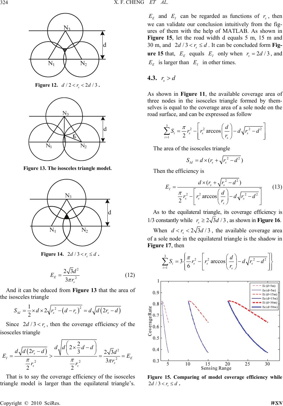

X. F. CHENG ET AL. 324
Figure 12. /22 /3
s
drd

.
Fsosceles triangle model. igure 13. The i
Figure 14. d2/3 s dr.
2
23d
2
3
E
s
Er

(12)
rom Figure 13 that the area of
the isosceles
And it can be educed f
triangle
 
2
2
122
2
Isss
Sdrdrddr
 
Since
d
2/3
s
dr, then the coverage efficiency of the
isosceles triangle

2
2
22
2323
3
2
2
2
2
s
I
E
s
s
d d
dd d
EE
r
rr





 
s
dd
r d


That is to say the coverage efficiency of the isosceles
triangle model is larger than the equilateral triangle’s.

E
E and
I
E can be regarded as functions of
s
r, then
we can validate our conclusion intuitively from the fig-
ures of them with the help of MATLAB. As shown in
Fiure 15, let the road width d equals 5 m, 15 m and
30 m, and d
g
2/3 s dr


at,
. It can be concluded form Fig-
ure 15 th
E
E equals
I
E only when , and 2/3
s
rd
E
E is larger than
I
E in other times.
4.3.
As shown in Figure 11, the available coverage area of
three nodes in the isosceles triangle formed by them-
selves is equal to the coverage area of a sole node on the
road surface, and can be expressed as follow
s
rd
3
22 22
12
iss s
is
r

arccos d Sr r drd




 

 






The area of the isosceles triangle
22
(
Iss
drrd  )S

Then the efficiency is
22
22 22
()
arccos
2
ss
I
ss s
s
drr d
E
d
rr drd
r

 






 



(13)
As to the equilateral triangle, its coverage efficiency is
1/3 constantly while 23/3
s
rd, as shown in Figure 16.
When 23 /3
s
dr d , the available coverage area
of a sole node in the equilateral triangle is the shadow in
Figure 17, then
3
22 22
1
3arccos
6
isss
is
Sr
r drd
r

d 







 



 









Figure 15. Comparing of model coverage efficiency while
2/3s drd

.

X. F. CHENG ET AL.325
Figure 16. The equilateral triangle model while=2 3 /3
s
rd .
Figure 17. The equilateral triangle model while <<
s
dr
23/3d.
=22 22 3arccos 3
2ss s
s
d
rr drd
r





And the efficiency is
2
3
3
E
d
E


22 22
3arccos 3
2ss s
s
rr drd
r




To compare them with each other, we also regard them
d
 (14)
as functions of
s
r, and plot them with the help of MAT-
LAB. As show Figure 18, let the road width d equals
5m, 15m and
n in
30m, and 3
s
dr d. It can be concluded
that

I
E is larger than
E
E, and
I
E approximates to 1 as
s
r increases, while
E
E approximates to 1/3.
5. Simulation Results
According to (9) and (10), it is clear that if the road
width d, sensor sensing range
s
r and the road length L
are given, then the number of sensor nodes required to
cover the road optimally can be calculated in determi-
nately deployment instance. In this section, we carry out
some simulated experiments based on our conclusions
with the help of MATLAB and C++, while d, L and
s
r
0). are varying. The calculating of n is based on (9) and (1
5.1. The Variance of n While One of d, L and
s
r
m
Changes
Figure 19 shows the variance of n while L increases fro
100m to 300m, in which d and
s
r is given. Accordi
(10), the two of them is linear, and the figure confirms
The slope of the line is , it is determined by (9).
Figure 20 shows the change of n while the sens
range of the sensor nodes increasing, in which d and
given. It can be made out from the figure that n is d
ng to
that.
ing
L is
e
/2l
-
creasing as
s
r increasing, and n approximates to 0 when
s
r is mucher than d.
Figure 21 shows the variance of n with d. We
clearly see that n goes to infinite when d approximates
double of
larg
can
to
s
r. According to (9) and (10), n is a subsec-
tion function and the inflexion comes while d = r, as th
figure reveals.
5.2. The Variance of n as Any Two of d, L
e
and
s
r Change
Figure 22 demonstrates the graph of n as L and
in which d = 20m. We can see that n is increasinwh
s
r
g
vary,
ile
s
r decreasing and L increasing, and n approxim
infinite when
ates to
s
r approximates to 10m that is half of t
road width.
that n approximates to
he
0
Figure 23 shows the graph of n varies with d ands r,
while L=300m. It is clearly
Figure 18. Comparing of model coverage efficiency while
3
s
drd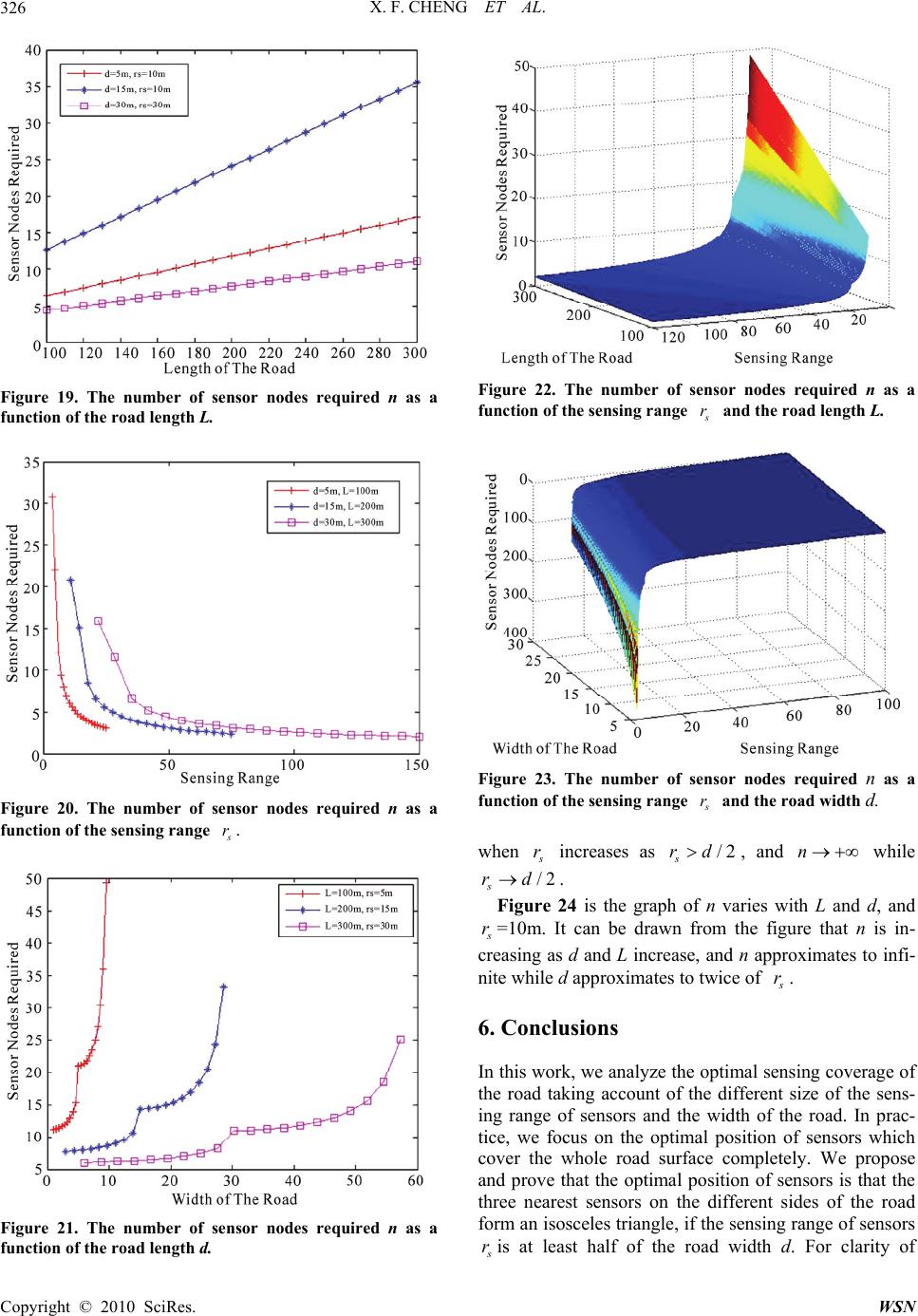

.

X. F. CHENG ET AL. 326
Figure 19. The number of sensor nodes required n as a
function of the road length L.
Figure 20. The number of ssor nodes required n asen a
nction of the sensing range fu
s
r.
Figure 22. The number of sensor nodes required n as a
function of the sensing range
s
r and the road length L.
Figure 23. The number of sensor nodes required n as a
function of the sensing range and the road width d.
s
r
Figure 21. The number of sensor nodes required n as a
function of the road length d.
when
s
r increases as /2
s
rd, and n while
/2
s
rd.
Figure 24 is the graph of n varies with L and d, and
s
r=10m. It can be drawn from the figure that n is in-
creasing as d and L increase, and n approximates to infi-
nite while d approximates to twice of
s
r.
6. Conclusions
In this work, we analyze th
the road taking account of
e optimal sensing coverage of
the different size of the sens-
es of the road
le, if the sensing range of sensors
ing range of sensors and the width of the road. In prac-
tice, we focus on the optimal position of sensors which
cover the whole road surface completely. We propose
and prove that the optimal position of sensors is that the
three nearest sensors on the different sid
form an isosceles triang
s
ris at least half of the road width d. For clarity of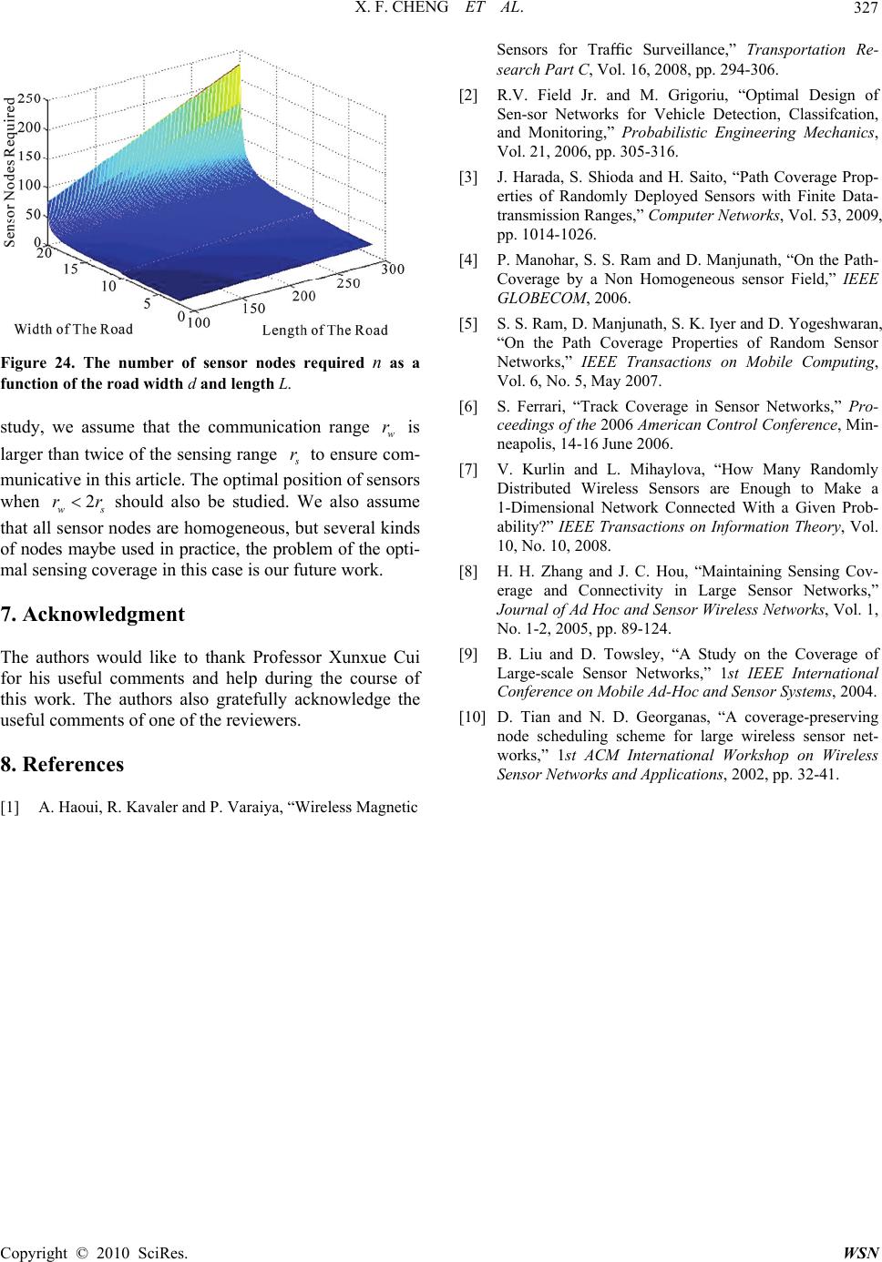

X. F. CHENG ET AL. 327
Figure 24. The number of sensor nodes required n as a
function of the road width d and length L.
study, we assume that the communication range is w r
larger than twice of the sensing range
s
r to ensure com-
municative in this article. The optimal position of sensors
n 2rrshould also bewhe
th
ws
studieWe also ase
at all sensor nodes are homogeneous, but several kinds
f nodes maybe used in practice, the problem of the opti-
al sensing coverage in this case is our future work.
. Acknowledgment
e authors would like to thank Professor Xunxue Cui
or his useful comments and help during the course of
is work. The authors also gratefully acknowledge the
useful comments of one of the reviewers.
8. References
[1] A. Haoui, R. Kavaler and P. Varaiya, “Wireless Magnetic
c Engineering Mechanics,
ting,
Vol. 6, No. 5, May 2007.
[6] S. Ferrari, “Track Coverage in Sensor Networks,” Pro-
ceedings of the 2006 American Control Conference, Min-
neapolis, 14-16 June 2006.
[7] V. Kurlin and L. Mihaylova, “How Many Randomly
Distributed Wireless Sensors are Enough to Make a
1-Dimensional Network Connected With a Given Prob-
ability?” IEEE Transactions on Information Theory, Vol.
10, No. 10, 2008.
[8] H. H. Zhang and J. C. Hou, “Maintaining Sensing Cov-
erage and Connectivity in Large Sensor Networks,”
Journal of Ad Hoc and Sensor Wireless Networks, Vol. 1,
No. 1-2, 2005, pp. 89-124.
[9] B. Liu and D. Towsley, “A Study on the Coverage of
Large-scale Sensor Networks,” 1st IEEE International
Conference on Mobile Ad-Hoc and Sensor Systems, 2004.
[10] D. Tian and N. D. Georganas, “A coverage-preserving
node scheduling scheme for large wireless sensor net-
works,” 1st ACM International Workshop on Wireless
Sensor Networks and Applications, 2002, pp. 32-41.
d. sum
Sensors for Traffic Surveillance,” Transportation Re-
search Part C, Vol. 16, 2008, pp. 294-306.
[2] R.V. Field Jr. and M. Grigoriu, “Optimal Design of
Sen-sor Networks for Vehicle Detection, Classifcation,
and Monitoring,” Probabilisti
Vol. 21, 2006, pp. 305-316.
[3] J. Harada, S. Shioda and H. Saito, “Path Coverage Prop-
erties of Randomly Deployed Sensors with Finite Data-
transmission Ranges,” Computer Networks, Vol. 53, 2009,
pp. 1014-1026.
[4] P. Manohar, S. S. Ram and D. Manjunath, “On the Path-
Coverage by a Non Homogeneous sensor Field,” IEEE
GLOBECOM, 2006.
[5] S. S. Ram, D. Manjunath, S. K. Iyer and D. Yogeshwaran,
“On the Path Coverage Properties of Random Sensor
Networks,” IEEE Transactions on Mobile Compu
o
m
7
Th
f
th