Wireless Sensor Network, 2010, 2, 285-292
doi:10.4236/wsn.2010.24039 Published Online April 2010 (http://www.SciRP.org/journal/wsn)
Data Discrimination in Fault-Prone Sensor Networks
Xiaoning Cui1,2,3,4,5, Qing Li4,5, Baohua Zhao1,2,3,4
1School of Computer Science and Technology, University of Science and Technology of China, Hefei, China
2State Key Laboratory of Networking and Switching Technology, Beijing, China
3Province Key Laboratory of Software in Computing and Communication, Hefei, China
4Joint Research Lab of Excellence, CityU-USTC Advanced Research Institute, Suzhou, China
5Department of Computer Science, City University of Hong Kong, Hong Kong, China
Received January 31, 2010; revised February 22, 2010; accepted February 24, 2010
Abstract
While sensor networks have been used in various applications because of the automatic sensing capability
and ad-hoc organization of sensor nodes, the fault-prone characteristic of sensor networks has challenged the
event detection and the anomaly detection which, to some extent, have neglected the importance of dis-
criminating events and errors. Considering data uncertainty, in this article, we present the problem of data
discrimination in fault-prone sensor networks, analyze the similarities and the differences between events
and errors, and design a multi-level systematic discrimination framework. In each step, the framework filters
erroneous data from the raw data and marks potential event samples for the next-step processing. The raw
data set D is finally partitioned into three subsets, Devent, Derro r and Dordina ry. Both the scenario-based simula-
tions and the experiments on real-sensed data are carried out. The statistical results of various discrimination
metrics demonstrate high distinction ratio as well as the robustness in different cases of the network.
Keywords: Data Discrimination, Fault-Prone Sensor Network, Event, Error, Distinction Ratio
1. Introduction
One of the major applications of sensor networks is event
detection [1], while the data uncertainty caused by faulty
sensors increases the difficulty of distinguishing between
events and errors in sensor data, and correspondingly
affects the design of data processing framework in a
sensor network. Due to the rather limited resource and
fault-prone characteristics in sensor networks, the design
principle of sensor data processing mainly lies in simple
operation, fault tolerance, distributed processing and
efficient distinction between erroneous measurements
and events [2,3]. The major techniques of anomaly de-
tection include histogram-based method [4], kernel esti-
mation [5,6], ranking/score-based method [7,8], depend-
ency analysis [9], and etc. There are also some extensive
research works on the region detection of anomalous
sensor readings [10,11]. However, to the best of our
knowledge, most of these works either separate event
detection and error detection into two problems or am-
biguously perceive events and errors as anomalies. Ac-
cording to the summary of the state-of-the-art anomaly
detection techniques [12], there lack sufficient concern
of the discrimination between events and errors in sensor
data processing [3]. Therefore, in this article, we focus
on designing a discrimination framework to solve this
problem.
The rest of the article is organized as follows. In Sec-
tion 2, the problem is analyzed based on the similarities
and differences between events and errors. In Section 3,
a discrimination framework is illustrated. The perform-
ance of the framework is evaluated by two scenario-
based simulations and a series of experiments on a
real-world sensor dataset in Section 4, and finally, Sec-
tion 5 concludes the article with some discussions on the
potential extension of the framework.
2. Problem Analysis
The problem of distinguishing between events and errors
has been investigated based on a few common assump-
tions [13]: 1) the network holds a hierarchical structure
and sensor data are forwarded to nearby local fusion
centers to handle data processing; 2) all of the data re-
ceived by the fusion center are not corrupted by any
communication fault; 3) there are no malicious attacks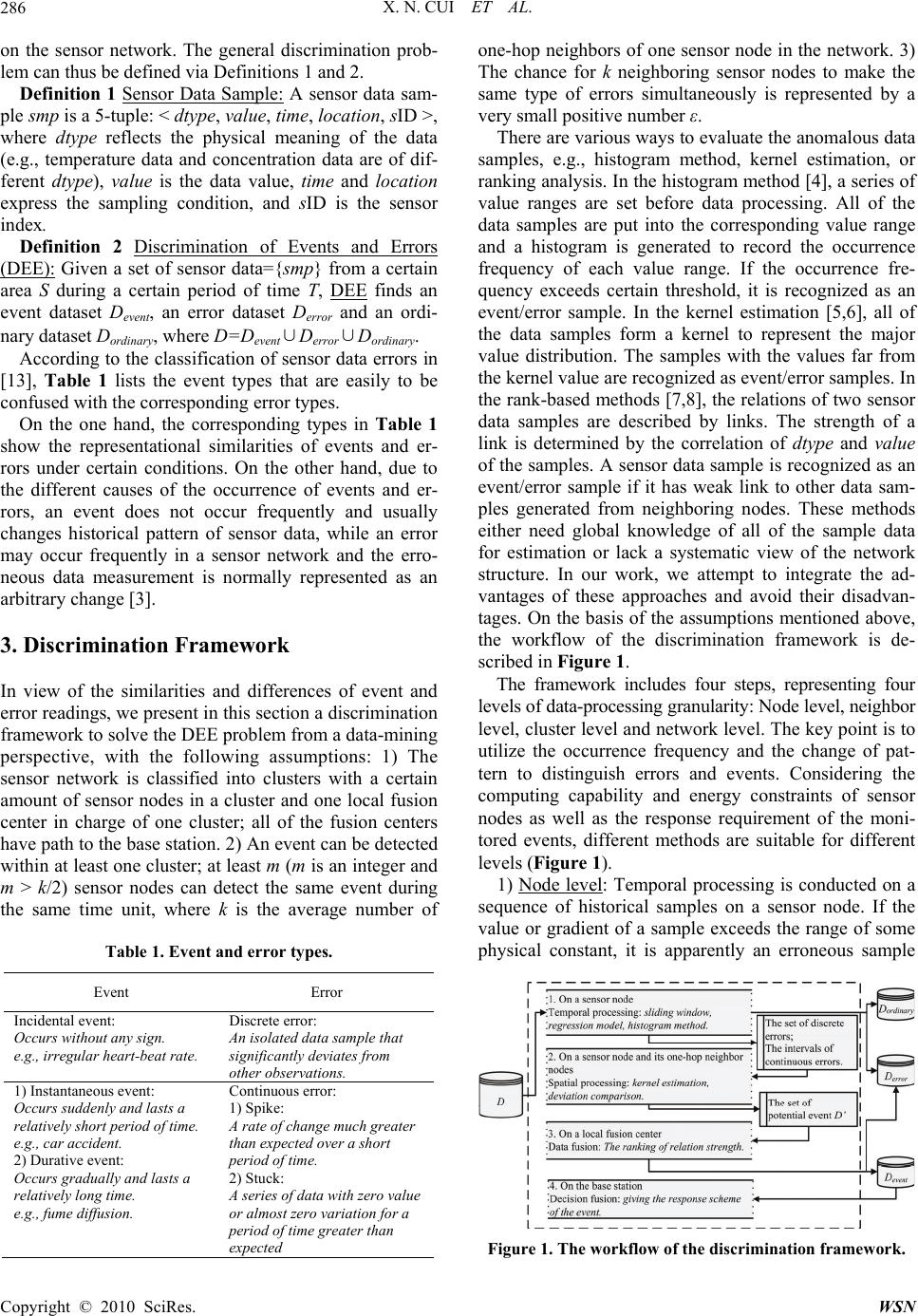

X. N. CUI ET AL. 286
on the sensor network. The general discrimination prob-
lem can thus be defined via Definitions 1 and 2.
Definition 1 Sensor Data Sample: A sensor data sam-
ple smp is a 5-tuple: < dtype, value, time, loca tion, sID >,
where dtype reflects the physical meaning of the data
(e.g., temperature data and concentration data are of dif-
ferent dtype), value is the data value, time and location
express the sampling condition, and sID is the sensor
index.
Definition 2 Discrimination of Events and Errors
(DEE): Given a set of sensor data={smp} from a certain
area S during a certain period of time T, DEE finds an
event dataset D
event, an error dataset D error and an ordi-
nary dataset Dordinary, where D=Devent∪Derror∪Dordinary.
According to the classification of sensor data errors in
[13], Table 1 lists the event types that are easily to be
confused with the corresponding error types.
On the one hand, the corresponding types in Table 1
show the representational similarities of events and er-
rors under certain conditions. On the other hand, due to
the different causes of the occurrence of events and er-
rors, an event does not occur frequently and usually
changes historical pattern of sensor data, while an error
may occur frequently in a sensor network and the erro-
neous data measurement is normally represented as an
arbitrary change [3].
3. Discrimination Framework
In view of the similarities and differences of event and
error readings, we present in this section a discrimination
framework to solve the DEE problem from a data-mining
perspective, with the following assumptions: 1) The
sensor network is classified into clusters with a certain
amount of sensor nodes in a cluster and one local fusion
center in charge of one cluster; all of the fusion centers
have path to the base station. 2) An event can be detected
within at least one cluster; at least m (m is an integer and
m > k/2) sensor nodes can detect the same event during
the same time unit, where k is the average number of
Table 1. Event and error types.
Event Error
Incidental event:
Occurs without any sign.
e.g., irregular heart-beat rate.
Discrete error:
An isolated data sample that
significantly deviates from
other observations.
1) Instantaneous event:
Occurs suddenly and lasts a
relatively short period of time.
e.g., car accident.
2) Durative event:
Occurs gradually and lasts a
relatively long time.
e.g., fume diffusion.
Continuous error:
1) Spike:
A rate of change much greater
than expected over a short
period of time.
2) Stuck:
A series of data with zero value
or almost zero variation for a
period of time greater than
expected
one-hop neighbors of one sensor node in the network. 3)
The chance for k neighboring sensor nodes to make the
same type of errors simultaneously is represented by a
very small positive number ε.
There are various ways to evaluate the anomalous data
samples, e.g., histogram method, kernel estimation, or
ranking analysis. In the histogram method [4], a series of
value ranges are set before data processing. All of the
data samples are put into the corresponding value range
and a histogram is generated to record the occurrence
frequency of each value range. If the occurrence fre-
quency exceeds certain threshold, it is recognized as an
event/error sample. In the kernel estimation [5,6], all of
the data samples form a kernel to represent the major
value distribution. The samples with the values far from
the kernel value are recognized as event/error samples. In
the rank-based methods [7,8], the relations of two sensor
data samples are described by links. The strength of a
link is determined by the correlation of dtype and value
of the samples. A sensor data sample is recognized as an
event/error sample if it has weak link to other data sam-
ples generated from neighboring nodes. These methods
either need global knowledge of all of the sample data
for estimation or lack a systematic view of the network
structure. In our work, we attempt to integrate the ad-
vantages of these approaches and avoid their disadvan-
tages. On the basis of the assumptions mentioned above,
the workflow of the discrimination framework is de-
scribed in Figure 1.
The framework includes four steps, representing four
levels of data-processing granularity: Node level, neighbor
level, cluster level and network level. The key point is to
utilize the occurrence frequency and the change of pat-
tern to distinguish errors and events. Considering the
computing capability and energy constraints of sensor
nodes as well as the response requirement of the moni-
tored events, different methods are suitable for different
levels (Figure 1).
1) Node level: Temporal processing is conducted on a
sequence of historical samples on a sensor node. If the
value or gradient of a sample exceeds the range of some
physical constant, it is apparently an erroneous sample
Figure 1. The workflow of the discrimination framework.

X. N. CUI ET AL.287
that should be put into Derror. Otherwise, the set of dis-
crete errors are picked out and the samples of continuous
errors are marked by interval for further processing. In
our work, linear regression is used based on a fixed size
of sliding window. The value differences of the predicted
samples and the real-sensed samples reflect the temporal
pattern of the sample sequence. Both events and errors
would incur significant change of pattern and thus a
higher value difference in prediction, according to which
the involved samples are marked for further discrimina-
tion. The rest of the samples are put into Dordinary.
2) Neighbor level: Spatial processing is used to com-
pare the samples with discrete errors or continuous errors
over neighboring nodes. Based on the assumptions in this
section, an anomalous sample probably reflects an event
if there is enough number (the number is set to be equal
to or over 50% in our simulation and experiment) of
neighboring nodes reporting the same data exception.
Such samples are put into the set of potential events D’.
Other anomalous samples belong to Derror.
3) Cluster level: The local fusion center evaluates the
samples in D' with reference to Dordinary. The event sam-
ples are finally selected from D' and constitute Devent. In
our work, we use deviation-based ranking strategy to
evaluate the samples in D' because it has been assumed
that there is little chance for all of the nearby nodes
(within a cluster) to get similar wrong readings. The
samples in D'\Devent are added to Derror.
4) Network level: The base station gets Devent and makes
decision fusion [14], i.e., taking action according to the
event information. Since it does not involve the DEE
problem, this level is beyond the scope of this paper.
4. Performance Evaluation
The performance of the discrimination framework is
evaluated by two scenario-based simulations in Subsec-
tion 4.1 and an experiment based on real-sensed data in
Subsection 4.2.
4.1. Scenario-Based Data Simulations
Scenario 1. Irregular heart-bit rate: The heart-bit rate
depicts how many times one’s heart beats per minute. A
human being usually keeps a stable heart-bit rate with
little fluctuations, represented as f(t) = c ± εc, where t is
the moment when measuring the heart-bit rate, c, and εc
is a small positive number to represent fluctuations. Ir-
regular heart-bit rate means that the fluctuation exceeds
the normal range, [–εc, εc]. The simulation based on Sce-
nario 1 aims at evaluating the performance on discrimi-
nating discrete errors with incidental events (Table 1).
Considering the requirement of the report correctness
and the response time, a small-scale network is simulated
with less than 10 sensor nodes. Meanwhile, the node-
level (Step 1) and neighbor-level (Step 2) processing are
employed in the data discrimination.
In Table 2, the error occurrence rate is the ratio of the
amount of erroneous samples over the total amount of the
samples. It is set from 10% to 50%, which is large enough
compared with the event occurrence rate (≤ 1%). This is
consistent with the frequency difference of errors and
events. A sample is recognized as either an ordinary sam-
ple or a potential-event sample in node-level processing,
except those which exceed the normal value range. The
neighbor level processing further discriminates events and
errors in the potential-event sample set. Therefore, c6 is
the distinction ratio in node-level processing (Step 1) and
the sum of r7, r8 and r9 is the distinction ratio in neighbor-
level processing (Step 2).
Given a set of sensor nodes measuring the heart-bit
rate of a person, the parameters are configured following
Table 2. Specifically, the simulations are conducted
through the following two cases.
Case 1. Slower heart-bit rate
Figure 2 shows the comparison of the distinction
Table 2. Parameter configuration of Scenario 1.
Parameters
General
parameters
Data amount: 1.44 × 107 heart-bit rate samples
per node with error/event injection;
Sampling frequency: 1kHz;
Error occurrence rate ≤ 50%;
Error type: discrete error;
Event occurrence rate ≤ 1%;
Event type: incidental event;
Normal heart-bit rate value range: [60,100];
Error/Event value range: [50,60) for slower
heart-bit rate and (100,199] for faster heart-bit
rate.
Step 1
(node level)
Window length: 4000 samples(data in 4
seconds);
Sliding ratio: 25% (1000 samples, data in 1
second).
Evaluation
metr i c s
(for Step1)
c1-mistaking errors for ordinary samples;
c2-marking errors as potential events;
c3-marking ordinary readings as potential
events;
c4-mistaking events for ordinary samples;
c5-marking events for potential events;
c6-correct distinction of ordinary samples;
c1 + c2 + c3+ c4 + c5 + c6 = 1;
Distinction ratio (Step 1) = c2.
Step 2
(neighbor level)Average number of 1-hop neighbors: 2
Evaluation
metr i c s
(for Step2)
r1-mistaking errors for ordinary samples;
r2-mistaking errors for events;
r3-mistaking ordinary readings for events;
r4-mistaking ordinary readings for errors;
r5-mistaking events for ordinary samples;
r6-mistaking events for errors;
r7-correct distinction of error samples;
r8-correct distinction of events samples;
r9-correct distinction of ordinary samples;
r1 + r2 + r3 + r4 + r5 + r6+ r7 + r8 + r9 = 1;
Distinction ratio (Step 2) = r7 + r8 + r9;
False Alarm = r2 + r3; Miss Hit = r5 + r6.

X. N. CUI ET AL. 288
Figure 2. Distinction ratio in each step of Case 1.
ratios after Steps 1 and 2. The distinction ratio after Step
1 declines with the increase of error occurrence rate, from
89.78% (when error occurrence rate = 10%) to 60.3 %
(when error occurrence rate = 50%). However, Step 2
achieves similar distinction ratio over 90% even though
the error occurrence rate is as high as 50%.
Moreover, as shown in Figure 3, the distinction ratios
of event and ordinary samples both approach 100%. The
distinction ratio of errors slightly goes down from 97%
(when error occurrence rate = 10%) to 84% (when error
occurrence rate = 50%).
Furthermore, Figure 4 shows the false-alarm rate and
the miss-hit rate for Case 1. On one hand, the false-alarm
rate grows larger with the increase of the error occur-
rence rate. The statistical result has shown that the in-
crease of error occurrence rate has accelerated the grow-
ing of the false-alarm rate. On the other hand, there is
almost no miss-hit in the data set.
Case 2. Faster heart-bit rate
Case 2 tests the performance on faster heart-beat rate
monitored by sensor networks. It is similar to Case 1,
except that the value ranges of event samples are differ-
ent. Figure 5 shows the step-wise comparison of the
distinction ratios. The trends are similar to that of Fig-
ure 2, i.e., the distinction ratio varies from 90.39%
(when error occurrence rate = 10%) down to 59.83%
(when error occurrence rate = 50%) after Step 1, and the
ratio increases to at least 93.31% after Step 2. When er-
ror occurrence rate =10%, such a ratio achieves as high
as 99.70%.
Figure 6 compares the distinction ratio of error sam-
ples, event samples and ordinary samples in Case 2.
Similarly to that in Case 1, the distinction ratio of errors
declines with the increase of erroneous data amount in
the data set, and the distinction of ordinary samples
keeps a stable ratio of near 100%. The event samples are
well discriminated under most conditions except when
error occurrence rate = 30%, where 1/6 event samples
are mistaken for error samples. This is because, in the
test case, many of the event samples are cross-occurred
with error samples within the same sliding window. It
means that the distinction ratio of event samples is not
affected by the error occurrence rate, but by when and
where an event and/or an error occur.
Figure 3. Comparison of distinction ratio of error (r7/(r1 + r2
+ r7)), event (r8/(r5 + r6 + r8)) and ordinary samples (r9/(r3 + r4
+ r9)) of Case 1.
0.17%
0.00%
Figure 4. False-alarm and miss-hit rate of Case 1.
Figure 5. Distinction ratio in each step of Case 2.
Figure 6. Comparison of distinction ratio of error, event
and ordinary samples of Case 2.
Figure 7 further gives the false-alarm rate and miss-
hit rate of Case 2. The values and trends are similar to
that in Case 1.
Scenario 2. Car accident: In the industry of car manu-
facture, accidents occur often due to acceleration. Ex-
perience tells that, when the sampling rate = 1 kHz and
the absolute acceleration (In the rest of this paper, we use
the word “acceleration” to represent “absolute accelera-

X. N. CUI ET AL.289
tion” for short.) exceeds 47 m/s2 between two consecu-
tive samples, car collision is expected to happen (see,
e.g., Figure 8 when time = 8 ms, acceleration = 50 m/s2).
Meanwhile, the response time of a car accident should be
less than 20ms so that the air bag could be triggered and
the driver could have enough time to take action.
There are usually 4 sensor nodes located at 4 wheels
of a car and a fusion center to integrate the samples, so
node-level (Step 1) and cluster-level (Step 2) processing
are employed in the simulation. Considering the change
pattern of the acceleration in Figure 8, an integra-
tion-based method is used in order to separate event
samples from erroneous samples, i.e., calculate the inte-
gration of the sample values within a sliding window
using Formula (1), and check whether the numerical in-
tegration exceeds a certain threshold:
1
1
(, )()
n
ink
Snk ai
f
 (1)
where f is the sampling rate, n is the total amount of sam-
ples and k is the window length. When f = 1 kHz and k is
set to 7 ms, the threshold is calculated by 0.5 × 7 × 47 =
164.5, indicating the linear changing process of the accel-
eration from 0 m/s2 to 47 m/s2 within a sliding window.
Similar to Table 2, Table 3 lists the parameter con-
figuration of the simulation.
Figure 9 compares the distinction ratio of error sam-
ples, event samples and ordinary samples of Scenario 2.
Since both the event pattern and the error types are more
complex in Scenario 2 than that in Scenario 1, the dis-
tinction ratios are generally lower than those in Scenario
1. However, the trends are the same, i.e., higher-level
processing will increase the distinction ratio.
0.08%
0.00%
Figure 7. False-alarm and miss-hit rate of Case 2.
Figure 8. The change pattern of the acceleration in a car
accident.
Table 3. Parameter configuration of Scenario 2.
Parameters
General
parameters
Data amount: 1000 acceleration samples
(1-second data) per node with error/event
injection;
Sampling frequency: 1kHz;
Error occurrence rate ≤ 50%;
Error type: Discrete and continuous errors;
Event occurrence rate ≤ 1%;
Event type: instantaneous event;
Normal acceleration range: [-2,2] (m/s2);
Error value range:[-100,100] (m/s2);
Event pattern: Following Figure 8.
Step 1
(node level)
Window length: 7 samples (data in 7ms);
Sliding ratio: 1/7 (data in 1ms).
Evaluation
metr i c s
(for Step1)
Distinction ratio (Step 1): The same as in
Table 2.
Step 2
(cluster level) The size of a fusion unit: 4 sensor nodes
Evaluation
metr i c s
(for Step2)
Distinction ratio (Step 2): Calculated by error
type.
Figure 9. Distinction ratio in each step of Scenario 2.
Furthermore, Figure 10 compares the distinction ratios
of discrete error (79.59% in average) and continuous error
(84.80% in average). It is shown that, the distinction ratio
varies with different error occurrence rate in the network,
but there is no significant sign to tell which type of errors
could be better discriminated in the data with a complex
event pattern. The performance of data discrimination
largely depends on the relative occurrence time and loca-
tion of errors and events. For example, in the test case,
when a continuous error occurs next to the event samples,
the processing tends to misjudge such erroneous samples.
Meanwhile, if most of the neighboring nodes are gener-
ating error samples, it is difficult for the fusion center to
report correct discrimination results.
4.2. Real-Sensed Data Experiment
Our experiment aims at testing the performance on the
discrimination of durative event samples. The experi-
ment is carried out based on the sensor data collected by
the Intel Berkeley Research Lab [15], where we select
the data generated from a subset of the sensor nodes and
inject errors and events to the raw data to evaluate the

X. N. CUI ET AL. 290
performance of the distinction framework. The experi-
ment includes three steps, corresponding to the process-
ing of the node, neighbor and cluster levels, respectively.
Without loss of generality, both the error probability of a
sample and the event pattern are unknown to a sensor
node. The parameters used in the experiment are listed in
Table 4.
The discrimination metrics in Table 4 are tested for
the sample prediction in Step 1 and the event discrimina-
tion of Steps 2 and 3. Figure 11 shows the accuracy
comparison of these metrics according to the experiment
on four nearby nodes (notes 1, 2, 3, and 33 in [15]) with
about 2000 temperature samples per node. Due to the
miss-sampling and over-sampling cases, the integrated
raw data have 2787 samples. The discrimination metrics
are calculated by sliding window. The correlation coeffi-
cient is shown as the best metric because of its stable
performance over both little-changed samples (e.g., the
samples during time intervals [2989, 3633], [4740, 5566])
and fast response over dynamically changed samples
(e.g., the samples during time interval [3689, 3904]).
Figure 10. The comparison of distinction ratios.
Table 4. Parameter configuration of the experiment.
Parameters
General
parameters
Data amount: 200 temperature samples per
node with error/event injection;
Error occurrence frequency ≤ 50%;
Event occurrence frequency ≤ 1%;
Error/Event value range: [-30, 100].
Step 1
(node level)
Window length: 40 samples;
Sliding ratio: 50%.
Step 2
(neighbor level) Average number of 1-hop neighbors: 3
Step 3
(cluster level) Average fusion range: 10 nearby nodes
Discrimination
metr i c s
Correlation coefficient, mean absolute error,
root mean squared error, relative absolute
error and root relative squared error.
Evaluation metrics
r1-mistaking errors for ordinary samples;
r2-mistaking errors for events;
r3-mistaking ordinary readings for events;
r4-mistaking ordinary readings for errors;
r5-mistaking events for ordinary samples;
r6-mistaking events for errors;
r7-correct distinction of events, errors, and
ordinary samples;
r1 + r2 + r3 + r4 + r5 + r6 + r7 = 1;
False Alarm = r2 + r3; Miss Hit = r5 + r6.
However, the other metrics are more or less inaccurate
over part of the samples. For example, except for the
correlation coefficient, all of the other four metrics show
fluctuations during time interval [5063, 5154] while the
raw samples do not change much during this time period.
Therefore, correlation coefficient is used to express the
value difference between the predicted and the real-
sensed samples.
The performance of the discrimination framework is
evaluated in different cases of error occurrence rate in
the network. The ratio r7 reflects how many samples are
correctly judged in each step over all of the samples. As
shown in Figure 12, r7 decreases with the increase of
error occurrence rate in Steps 1 and 2, but Step 3 has
corrected most of the wrong discriminations and kept the
ratio as high as 97% in all of the five cases. Meanwhile,
Figure 13 shows that, in different cases of the network,
the step-wise processing has always kept an increasing
Figure 11. The comparison of different distinction metrics.
Figure 12. The comparison of different steps in processing.
Figure 13. The comparison of different error occurrence
frequency.

X. N. CUI ET AL.291
trend of the correct distinction (i.e., r7), demonstrating
the robustness of the discrimination framework.
Besides the ratio of correct distinction, the ratios of
false alarm and miss hit have been analyzed in Figure 14.
Although the false alarm is relatively high in the first
step, the processing of the following two steps can sig-
nificantly reduce the ratio of false alarm. The average
false-alarm rates after each step are 9%, 0.6% and 0.5%.
On the other hand, the average miss-hit rates after each
step are 0.5%, 0.8% and 0.6%. There is slight increase of
miss-hit rate after Steps 2 and 3. This is because new
errors would be incurred by the cross-comparison and
ranking among samples from different nodes. Thus,
tradeoffs exist between the false-alarm rate and miss-hit
rate in the discrimination framework.
More specifically, there are usually higher false-alarm
rates in the solutions to event-detection problems since
they mistake erroneous samples for event samples. On
the other hand, the approaches of traditional anom-
aly-detection problems often mistake event samples for
erroneous samples and result in higher miss-hit rates.
Figure 15 and Figure 16 compare the false-alarm rate
Figure 14. Statistical result of false alarm and miss hit.
Figure 15. Comparison of false-alarm rate.
Figure 16. Comparison of miss-hit rate.
and miss-hit rate of the discrimination framework for
DEE problem with the corresponding methods in event
detection and anomaly detection, respectively. It is ob-
vious that the discrimination framework in our work has
significantly outperformed the traditional event-detection
method in false-alarm rate, and the miss-hit rate of the
discrimination framework is much lower than that of the
traditional anomaly-detection framework.
5. Conclusions and Future Work
Different from the traditional event detection and anom-
aly detection problems, in this article, we have presented
the problem of data discrimination to separate sensor
data into the subsets of error samples, event samples and
ordinary samples. A multi-level processing framework
has been devised in view of the characteristics and con-
straints of sensor nodes, as well as the requirement of
discrimination correctness and response time. Both the
scenario-based simulations and the experiment based on
real-sensed data have been carried out to evaluate the
performance of the discrimination framework. The
simulation and experimental results show that different
types of monitored events need different kinds of
data-discrimination methods and different level of data
processing. For example, the correlation coefficient serves
as the most appropriate distinction metric in the sample
discrimination of durative events. According to the
comparison results of false-alarm and miss-hit rate of
the methods for traditional event-detection and anom-
aly-detection problems, the multi-level processing frame-
work has significantly increased the correct distinction
ratio, substantially reduced the false-alarm rate, and kept
the miss-hit rate in an acceptable low level.
In the future, we plan to apply such a framework to
more specific event monitoring problems in fault-prone
sensor networks. It is believed that good performance of
data discrimination comes from wise use of the do-
main-knowledge of the event patterns and error patterns
as well as the characteristics of wireless sensor networks.
6. References
[1] D. Shepherd and S. Kumar, “Microsensor Applications,”
In: S. S. Iyengar and R. R. Brooks Eds., Distributed Sen-
sor Networks, Chapman & Hall/CRC Press, 2005, pp. 11-27.
[2] P. Buonadonna, D. Gay, J. M. Hellerstein, W. Hong and
S. Madden, “TASK: Sensor Network in a Box,” Techni-
cal Report, International Research Berkeley, January
2005.
[3] Y. Zhang, M. Nirvana and H. Paul. “Why General Outlier
Detection Techniques Do Not Suffice for Wireless Sensor
Networks?” Intelligent Techniques for Warehousing and
Mining Sensor Network Data, IGI Global, 2009.
[4] B. Sheng, Q. Li, W. Z. Mao and W. Jin. “Outlier Detec-
tion in Sensor Networks,” Proceedings of the ACM Inter-

X. N. CUI ET AL. 292
national Symposium on Mobile Ad Hoc Networking and
Computing, Montreal, September 2007, pp. 219-228.
[5] T. Palpanas, D. Papadopoulos, V. Kalogeraki and D.
Gunopulos, “Distributed Deviation Detection in Sensor
Networks,” SIGMOD Record, Vol. 32, No. 4, December
2003, pp. 77-82.
[6] S. Subramaniam, T. Palpanas, D. Papadopoulos, V. Ka-
logeraki and D. Gunopulos, “Online Outlier Detection in
Sensor Data Using Non-Parametric Models,” Proceed-
ings of Very Large Data Bases, Seoul, 12-15 September
2006, pp. 187-198.
[7] J. W. Branch, C. Giannella, B. Szymanski, R. Wolff and
H. Kargupta. “In-network Outlier Detection in Wireless
Sensor Networks,” Proceedings of 26th International
Conference on Distributed Computing Systems, Lisboa,
4-7 July 2006.
[8] M. E. Otey, A. Ghoting and S. Parthasarathy. “Fast Dis-
tributed Outlier Detection in Mixed-Attribute Data Sets,”
International Journal of Data Mining and Knowledge
Discovery, Vol. 12, No. 2-3, 2006, pp. 203-228.
[9] D. Janakiram, V. Reddy and A. Kumar, “Outlier Detec-
tion in Wireless Sensor Networks Using Bayesian Belief
Networks,” 1st International Conference on Communica-
tion System Software and Middleware, New Delhi, 2006,
pp. 1-6.
[10] C. Franke and M. Gertz, “ORDEN: Outlier Region De-
tection and Exploration in Sensor Networks,” Proceed-
ings of ACM Special Interest Group on Management of
Data, Providence, 29 June-2 July 2009.
[11] M. Ding, D. C. Chen, K. Xing and X. Z. Cheng. “Local-
ized Fault-Tolerant Event Boundary Detection in Sensor
Networks,” Proceedings of 24th Annual Joint Conference
of the IEEE Computer and Communications Societies,
Vol. 2, 13-17 March 2005, pp. 902-913.
[12] V. Chandola, A. Banerjee and V. Kumar, “Anomaly De-
tection: A Survey,” ACM Computing Surveys, September
2009, pp. 1-72.
[13] K. Ni, N. Ramanathan, M. N. H. Chehade, L. Balzano, S.
Nair, S. Zahedi, E. Kohler, G. Pottie, M. Hansen and M.
Srivastava, “Sensor Network Data Fault Types,” ACM
Transactions on Sensor Networks, Vol. 5, No. 3, May 2009.
[14] M. M. Kokar, J. A. Tomasik and J. Weyman, “Data vs.
Decision Fusion in the Category Theory Framework,”
Proceedings of Fusion 4th International Conference on
Information Fusion, Vol. 1, 2001.
[15] http://db.csail.mit.edu/labdata/labdata.html