Engineering, 2010, 2, 190-196
doi:10.4236/eng.2010.23027 lished Online March 2010 (http://www.SciRP.org/journal/eng/)
Pub
The Effect of Near-Wall Vortices on Wall Shear Stress in
Turbulent Boundary Layers
Shuangxi Guo1, Wanping Li2
1School of Civil Engineering and Mechanics, Huazhong University of Science and Technology, Wuhan, China
2The Key Laboratory of Mechanics on Western Disaster and Environment of the Ministry of Education of China,
Lanzhou, China
Received June 10, 2009; revised July 9, 2009; accepted July 21, 2009
Abstract
The objective of the present study is to explore the relation between the near-wall vortices and the shear
stress on the wall in two-dimensional channel flows. A direct numerical simulation of an incompressible
two-dimensional turbulent channel flow is performed with spectral method and the results are used to exam-
ine the relation between wall shear stress and near-wall vortices. The two-point correlation results indicate
that the wall shear stress is associated with the vortices near the wall and the maximum correlation-value lo-
cation of the near-wall vortices is obtained. The analysis of the instantaneous diagrams of fluctuation veloc-
ity vectors provides a further expression for the above conclusions. The results of this research provide a
useful supplement for the control of turbulent boundary layers.
Keywords: Spectral Methods, Two-Dimensional Turbulence, Wall Shear Stress, Two-Point Correlation
1. Introduction
The flow phenomenon of turbulent boundary layers is
common in nature. It is closely related to aerospace, ma-
rine, environmental energy, chemical engineering and
other fields. In aeronautical engineering, the complex
turbulent vortex structures in boundary layers not only
affect the working stability and security of the aircraft
but also increase the skin friction on the wall remarkably.
So the research of control of turbulent boundary layers is
significant. In recent years the related literatures focus
mainly on two aspects: control of near-wall turbulent
structures and wall skin friction. Essentially, the wall
skin friction is closely related with the near-wall turbu-
lent structures, so the researches on these two aspects are
in accordance. In flat wall flows, the wall shear stress
constitutes wall skin friction. Sheng, Malkiel and Katz
did much in-depth and complete study on the relation
between wall shear stress (streamwise and spanwise) and
near-wall flow structure (streamwise, spanwise and out-
side structure) by experiment method [1]. Most re-
searchers agreed that the near-wall streamwise vortices
were the main effect factors of wall shear stress [2-5].
The wall normal and spanwise velocities boundary con-
ditions were presented by the methods of wall blowing
and suction or spanwise-wall oscillation, which directly
changed the near-wall streamwise vortices and achieved
the purpose of control of the wall shear stress [6-8].
Though the detailed mechanism has not been completely
clear so far, the above-mentioned control methods have
made good effectiveness on wall shear stress reduction.
Recently Y. S. Park et al also researched the control of
wall shear stress by the method of wall blowing and suc-
tion. Instead of vertical to the wall, certain angles were
presented between the blowing-suction direction and the
streamwise direction. This meant that the velocity
boundary conditions brought by their control method
were normal and streamwise velocities instead of normal
and spanwise velocities. Their experiments showed a
better effectiveness of wall shear stress reduction if the
angle was proper [9]. In fact, wall normal and stream-
wise velocity boundary conditions changed the near-wall
spanwise vortices directly. As well as streamwise vor-
tices, spanwise vortices are also the main characteristics
in turbulent boundary layers, while are they also the cru-
cial effect factors on wall shear stress as the streamwise
vortices?
Essentially, turbulent flow is absolutely three-dimen-
sional, but some certain turbulence motion, such as at-
mosphere or ocean flows, is behaving quasi-two-dimen-
sionally. The horizontal scales are hundreds of kilome-
ters in the ocean and thousands of kilometers in the at-

S. X. Guo ET AL. 191
mosphere, while their vertical scale is only a few kilo-
meters. So the turbulent motions in the vertical direction
are suppressed and can be ignored can be treated as two-
dimensional turbulence [10-11]. The saturation states of
two-dimensional turbulence have the similar characteris-
tics as the three-dimensional turbulence, such as injec-
tion, sweep and other bursting phenomenon [12-13],
while they have lots of differences from the three-di-
mensional turbulence, such as self-organization and in-
verse energy cascade [10-11]. In addition, the simulation
of two-dimensional turbulence requires less expensive
computational resources in comparison with that of
three-dimensional turbulence. So it is also valuable for
the study of two-dimensional turbulence. Moreover, sca-
lar vorticity in two-dimensional turbulence is controlled
by the normal and streamwise velocity, and has the same
expression as the spanwise vorticity in three-dimensional
turbulence, 


vu
x
y
 . So in the present paper the
two-dimensional scalar vorticity is taken as the major
subject of study instead of the three-dimensional span-
wise vorticity. The objective of the present study is to
explore the relation between the near-wall vortices and
the shear stress on the wall in two-dimensional channel
flows.
So far, the researches of two-dimensional turbulence
are mainly limited to the models with unbounded condi-
tion, or with the identical bounded condition such as squ-
are or circular domains. The literatures of two-dimens-
ional channel flow are rare. W. Kramer, H. J. H. Clercx
and G. J. F. van Heijst have done some pioneering study
on this subject. They have researched the influence of the
aspect ratio of the channel and the integral-scale Rey-
nolds number on the large-scale self-organization of the
flow in detail and obtained lots of important consequence
[11]. In the present paper, the numerical process to
simulate the two-dimensional turbulent channel flows
directly with spectral method is firstly introduced, and
the accuracy and stability of the proposed algorithm is
verified with two examples. Secondly the relation be-
tween the wall shear stress and near-wall vortices is ex-
plored and the maximum correlation-value location of
the near-wall vortices is obtained. Finally the instanta-
neous diagrams of fluctuation velocity vectors and the
near-wall model are analyzed to provide a further ex-
pression for the conclusions obtained.
2．Numerical Processes
2.1. Numerical Method
With the development of computational technology and
resources, the direct numerical simulation (DNS) is more
and more widely used as the basic research approach of
turbulence. Spectral method is one of the most common
methods for the DNS of turbulence, which has many
advantage, such as high degree of accuracy, quickly
speed on convergence, and analytically spatial derivation
for flow variables [13]. Many researchers have done lots
of pioneering and significant achievements for this
method, such as John Kim, Moin & Moser [14], Kleiser
& Schumann [15], Hu, Morfey & Sandham [16]. So
spectral method is applied to solve the Navier-Stokes
equation directly in the present study.
The governing equations for two-dimensional incom-
pressible channel flow can be written as the following
forms:
2
1
Re

 

i
ii
i
up
f
u
tx (1)
0



i
i
u
x (2)
Here, all variables are non-dimensionalized by the
channel half-width

and laminar Poiseuille flow cen-
tral velocity ; Non-linear term
c
Ui
f
includes the con-
vective terms and the mean pressure gradient [14]; and
denotes the Reynolds number defined as Re Re /
c
U


 ,
where

is kinematic viscosity.
Vorticity

is defined as 


vu
x
y
 . Equation (1)
can be reduced to yield a second-order equation for the
vorticity as follows:
23
1
1
Re
  


f
f
tz

x
(3)
The velocity component equations can be deduced due
to

and continuity Equation (2):
2



uy

, 2


v
x

(4)
Fully developed turbulent channel flow is homogene-
ous in the streamwise direction, and periodic boundary
conditions are used in this direction. All unknown quan-
tities are expanded with Fourier series in the streamwise
direction and Chebyshev polynomial in the normal direc-
tion as follows:

12
1
/2
/2 0
(,,)() exp()()


NN
mp mp
mN P
qxytqtixTy 
where

mm

 .

is amount of streamwise period,
defined as 2/

n
x

 , n
x
is the non-dimensional width
of computational domain in the streamwise direction;
is streamwise wave number; is p-order Cheby-
shev polynomial.
m
()
p
Ty
C opyright © 2010 SciRes. ENG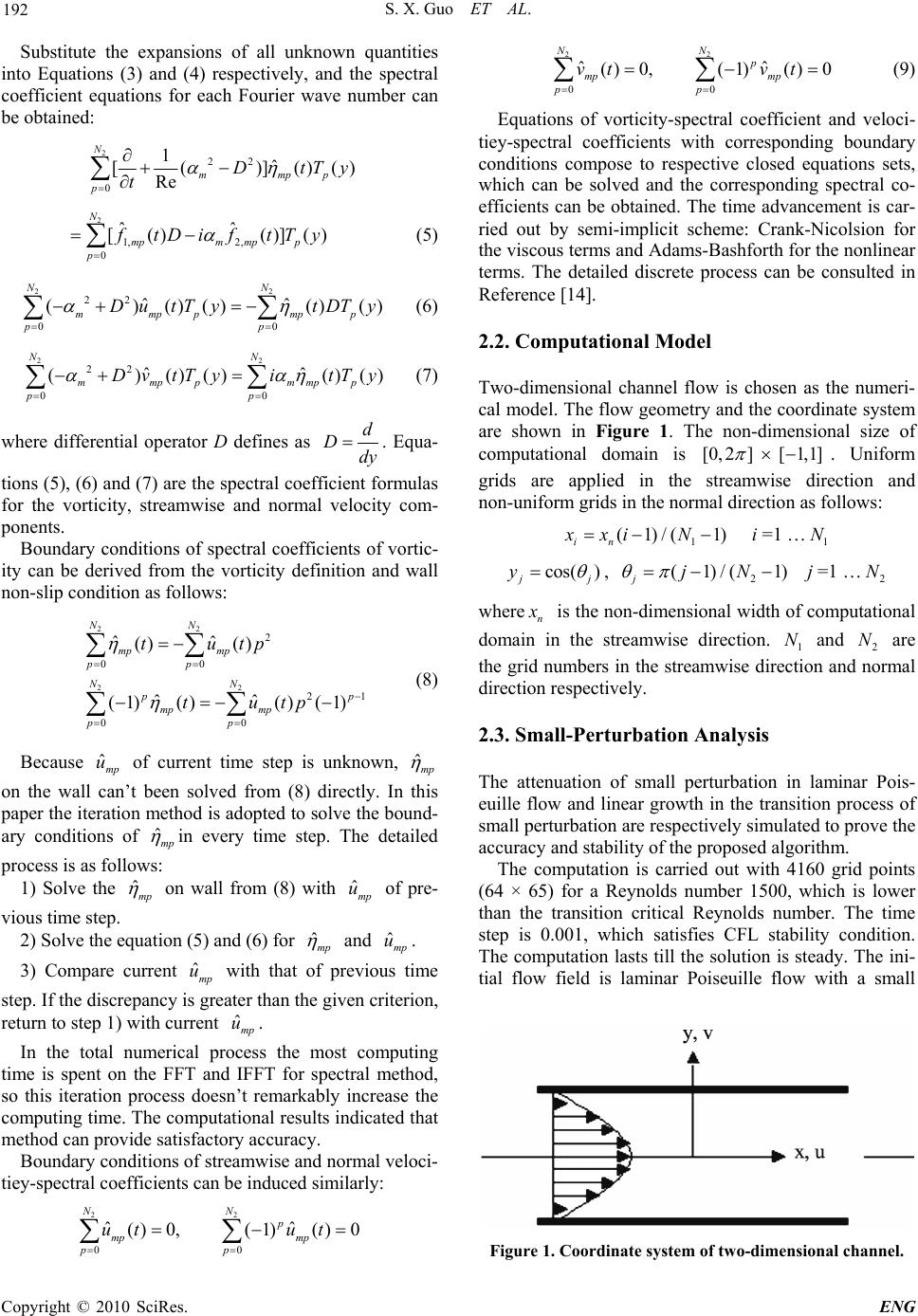

S. X. Guo ET AL. 192
Substitute the expansions of all unknown quantities
into Equations (3) and (4) respectively, and the spectral
coefficient equations for each Fourier wave number can
be obtained:
2
22
0
1ˆ
[( )]()
Re




N
mmpp
p
DtT
t
 ()y
)
2
1, 2,
0
ˆˆ
[() ()](



N
mpm mpp
p
f
tDift Ty  (5)
22
22
00
ˆ ˆ
()()()()( )

 

NN
mmpp mpp
pp
Du tTytDTy  (6)
22
22
00
ˆ ˆ ()()() ()

 

NN
mmpp mmpp
pp
Dv tTyitTy  ()  (7)
where differential operator D defines as d Ddy. Equa-
tions (5), (6) and (7) are the spectral coefficient formulas
for the vorticity, streamwise and normal velocity com-
ponents.
Boundary conditions of spectral coefficients of vortic-
ity can be derived from the vorticity definition and wall
non-slip condition as follows:
22
22
2
00
21
00
ˆˆ () ()
ˆˆ
(1)()()(1)







NN
mp mp
pp
NN
p
p
mp mp
pp
tutp
tutp


(8)
Because of current time step is unknown,
ˆmp
uˆmp

on the wall can’t been solved from (8) directly. In this
paper the iteration method is adopted to solve the bound-
ary conditions of ˆmp

in every time step. The detailed
process is as follows:
1) Solve the ˆmp

on wall from (8) with of pre-
vious time step.
ˆmp
u
2) Solve the equation (5) and (6) for ˆmp

and .
ˆmp
u
3) Compare current with that of previous time
step. If the discrepancy is greater than the given criterion,
return to step 1) with current .
ˆmp
u
ˆmp
u
In the total numerical process the most computing
time is spent on the FFT and IFFT for spectral method,
so this iteration process doesn’t remarkably increase the
computing time. The computational results indicated that
method can provide satisfactory accuracy.
Boundary conditions of streamwise and normal veloci-
tiey-spectral coefficients can be induced similarly:
22
00
ˆˆ ()0, (1)()0



NN
p
mp mp
pp
ut ut
22
00
ˆˆ ()0, (1)()0




NN
p
mp mp
pp
vt vt (9)
Equations of vorticity-spectral coefficient and veloci-
tiey-spectral coefficients with corresponding boundary
conditions compose to respective closed equations sets,
which can be solved and the corresponding spectral co-
efficients can be obtained. The time advancement is car-
ried out by semi-implicit scheme: Crank-Nicolsion for
the viscous terms and Adams-Bashforth for the nonlinear
terms. The detailed discrete process can be consulted in
Reference [14].
2.2. Computational Model
Two-dimensional channel flow is chosen as the numeri-
cal model. The flow geometry and the coordinate system
are shown in Figure 1. The non-dimensional size of
computational domain is [0,2] [1,1]

 . Uniform
grids are applied in the streamwise direction and
non-uniform grids in the normal direction as follows:
1
(1)/( 1)


in
xxi N =1 … i1 N
cos( )

jj
y

, 2 (1)/( 1)


jjN

 =1 …
j2
N
wheren
x
is the non-dimensional width of computational
domain in the streamwise direction. and are
the grid numbers in the streamwise direction and normal
direction respectively.
1
N2 N
2.3. Small-Perturbation Analysis
The attenuation of small perturbation in laminar Pois-
euille flow and linear growth in the transition process of
small perturbation are respectively simulated to prove the
accuracy and stability of the proposed algorithm.
The computation is carried out with 4160 grid points
(64 × 65) for a Reynolds number 1500, which is lower
than the transition critical Reynolds number. The time
step is 0.001, which satisfies CFL stability condition.
The computation lasts till the solution is steady. The ini-
tial flow field is laminar Poiseuille flow with a small

Figure 1. Coordinate system of two-dimensional channel.

S. X. Guo ET AL. 193
perturbation. Figure 2(a) shows the deviation between
initial flow field and Poiseuille flow. Figure 2(b) shows
that the profile of steady velocity solution is consistent
(a)
(b)
(c)
Figure 2. (a) Contrast between initial velocity profile and
Poiseuille profile; (b) contrast between solved steady veloc-
ity profile and Poiseuille profile; (c) variation of maximal
deviation with time between computational flow field and
Poiseuille flow, the figure inside is partial magnification
(
p
uand are the computational streamwise velocity and
Poiseuille velocity).
a
u
with that of Poiseuille flow. Figure 2(c) shows the varia-
tion of maximal deviation with time between computa-
tional flow field and Poiseuille flow. It can be seen that
the maximal deviation gradually reduces and approxi-
mately equals zero, even less than . Computational
results reflect the attenuation of small perturbation in
laminar flow and prove the accuracy and stability of the
proposed algorithm.
8
10
The Reynolds number is increased to 7500, which is
higher than the transition critical Reynolds number. The
objective is to calculate the linear growth rate of small
perturbation with the proposed algorithm in this paper
and compare that with the results by solving the Orr-
Sommerfield equation. The initial flow field with small
perturbation is set as follows:
2
(, )1,  uxyy u

(,) vxy v

where and are in accordance with the most insta-
ble model of stability theory with the perturbation wave
number

u v
01.


and amplitude 0.0001

＝. Kinetic
ene- rgy of perturbation is defined as:
12 22
10
()()


 
E tuvdxdy

According to the linear theory of small perturbation,
the kinetic energy increases exponentially with time,
. The linear growth rate c is 0.004470 by
solving the Orr-Sommerfield equation. Figure 3 shows
that the computational results of kinetic energy of per-
turbation with the proposed algorithm in present paper
are in good agreement with the theoretical ones by solv-
ing the Orr-Sommerfield equation.
() (0)ct EtE e
3. Wall Shear Stress Analysis
Y. S. Park et al. investigated the effect of periodic blow-
ing and suction on a turbulent boundary layer at three
different blowing-suction angles (60 , and 120 )
90 
Figure 3. Linear growth of small perturbation.
C opyright © 2010 SciRes. ENG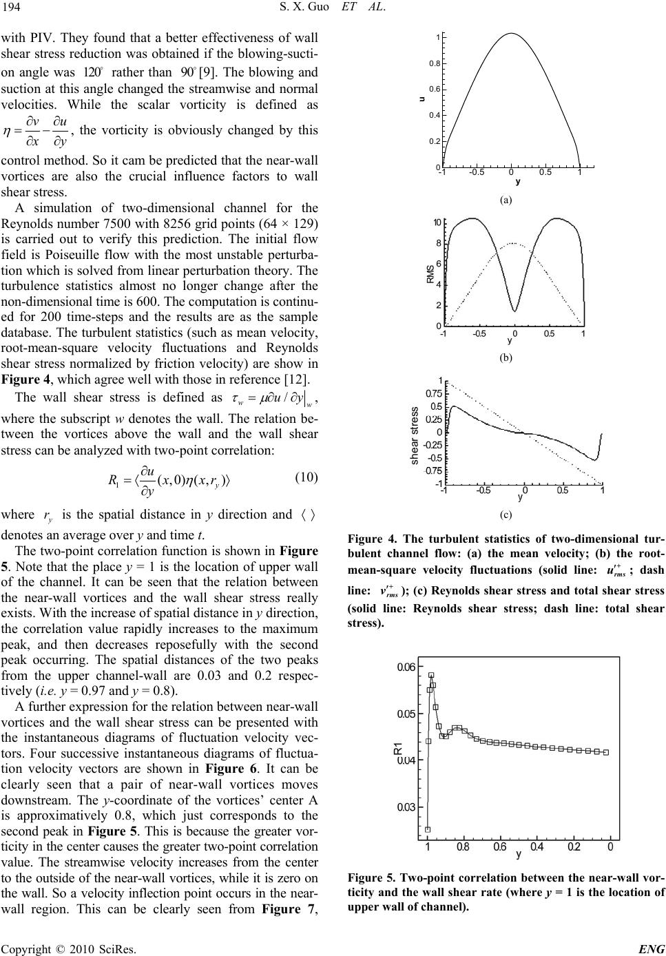

S. X. Guo ET AL. 194
with PIV. They found that a better effectiveness of wall
shear stress reduction was obtained if the blowing-sucti-
on angle was rather than [9]. The blowing and
suction at this angle changed the streamwise and normal
velocities. While the scalar vorticity is defined as
12090



vu
x
y
 , the vorticity is obviously changed by this
control method. So it cam be predicted that the near-wall
vortices are also the crucial influence factors to wall
shear stress.
A simulation of two-dimensional channel for the
Reynolds number 7500 with 8256 grid points (64 × 129)
is carried out to verify this prediction. The initial flow
field is Poiseuille flow with the most unstable perturba-
tion which is solved from linear perturbation theory. The
turbulence statistics almost no longer change after the
non-dimensional time is 600. The computation is continu-
ed for 200 time-steps and the results are as the sample
database. The turbulent statistics (such as mean velocity,
root-mean-square velocity fluctuations and Reynolds
shear stress normalized by friction velocity) are show in
Figure 4, which agree well with those in reference [12].
The wall shear stress is defined as / 
ww
uy  ,
where the subscript w denotes the wall. The relation be-
tween the vortices above the wall and the wall shear
stress can be analyzed with two-point correlation:
1(,0)(, ) y
u
Rxxr
y


 
 (10)
where is the spatial distance in y direction and
y
r


denotes an average over y and time t.
The two-point correlation function is shown in Figure
5. Note that the place y = 1 is the location of upper wall
of the channel. It can be seen that the relation between
the near-wall vortices and the wall shear stress really
exists. With the increase of spatial distance in y direction,
the correlation value rapidly increases to the maximum
peak, and then decreases reposefully with the second
peak occurring. The spatial distances of the two peaks
from the upper channel-wall are 0.03 and 0.2 respec-
tively (i.e. y = 0.97 and y = 0.8).
A further expression for the relation between near-wall
vortices and the wall shear stress can be presented with
the instantaneous diagrams of fluctuation velocity vec-
tors. Four successive instantaneous diagrams of fluctua-
tion velocity vectors are shown in Figure 6. It can be
clearly seen that a pair of near-wall vortices moves
downstream. The y-coordinate of the vortices’ center A
is approximatively 0.8, which just corresponds to the
second peak in Figure 5. This is because the greater vor-
ticity in the center causes the greater two-point correlation
value. The streamwise velocity increases from the center
to the outside of the near-wall vortices, while it is zero on
the wall. So a velocity inflection point occurs in the near-
wall region. This can be clearly seen from Figure 7,
-1-0.500.5 1
y
0
0.2
0.4
0.6
0.8
1
u
(a)
(b)
shear stress
(c)
Figure 4. The turbulent statistics of two-dimensional tur-
bulent channel flow: (a) the mean velocity; (b) the root-
mean-square velocity fluctuations (solid line:

+
rms
u; dash
line:

+
rms
v); (c) Reynolds shear stress and total shear stress
(solid line: Reynolds shear stress; dash line: total shear
stress).
Figure 5. Two-point correlation between the near-wall vor-
ticity and the wall shear rate (where y = 1 is the location of
upper wall of channel).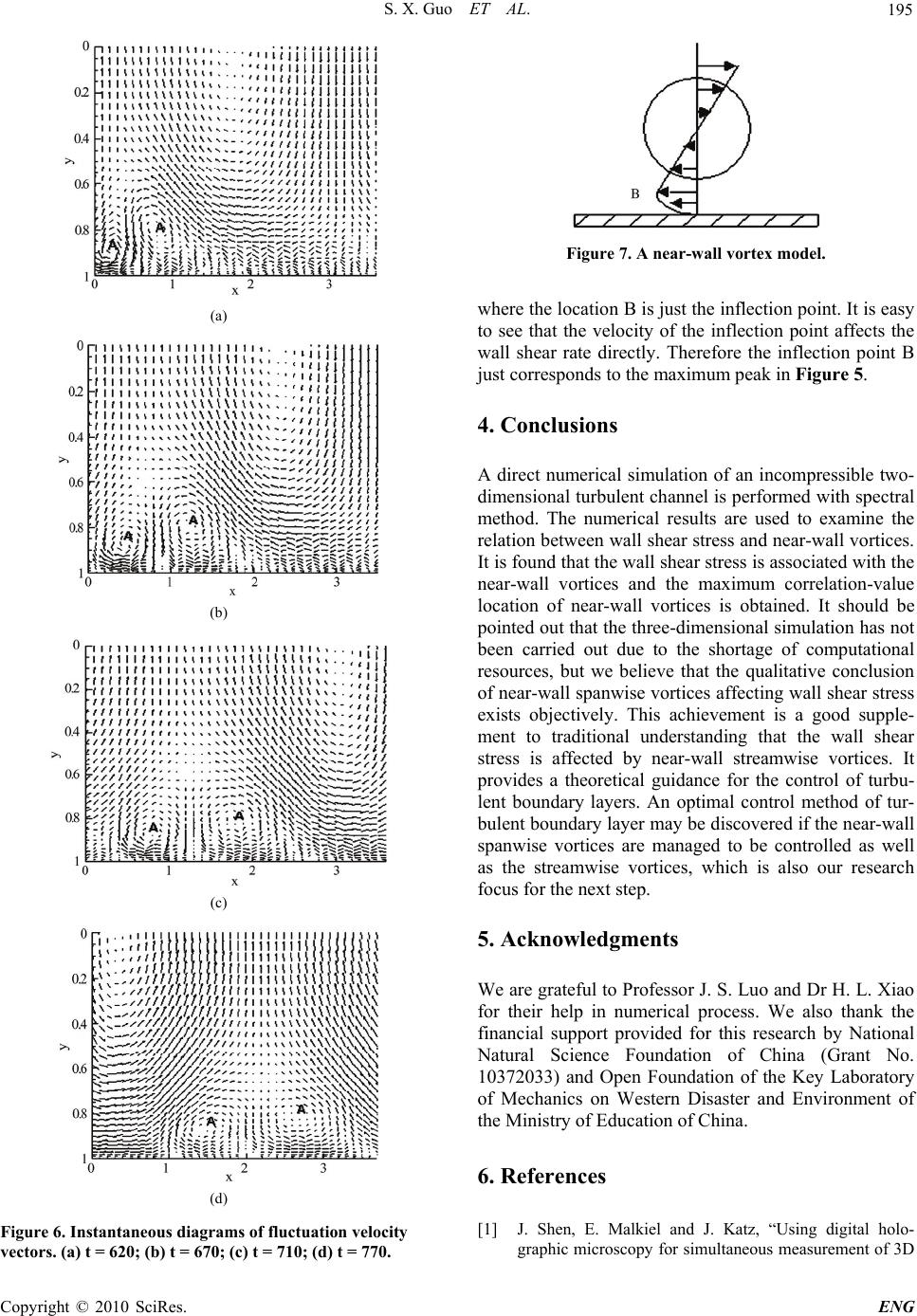

S. X. Guo ET AL. 195
(a)
(b)
(c)
(d)
Figure 6. Instantaneous diagrams of fluctuation velocity
vectors. (a) t = 620; (b) t = 670; (c) t = 710; (d) t = 770.
Figure 7. A near-wall vortex model.
where the location B is just the inflection point. It is easy
to see that the velocity of the inflection point affects the
wall shear rate directly. Therefore the inflection point B
just corresponds to the maximum peak in Figure 5.
4. Conclusions
A direct numerical simulation of an incompressible two-
dimensional turbulent channel is performed with spectral
method. The numerical results are used to examine the
relation between wall shear stress and near-wall vortices.
It is found that the wall shear stress is associated with the
near-wall vortices and the maximum correlation-value
location of near-wall vortices is obtained. It should be
pointed out that the three-dimensional simulation has not
been carried out due to the shortage of computational
resources, but we believe that the qualitative conclusion
of near-wall spanwise vortices affecting wall shear stress
exists objectively. This achievement is a good supple-
ment to traditional understanding that the wall shear
stress is affected by near-wall streamwise vortices. It
provides a theoretical guidance for the control of turbu-
lent boundary layers. An optimal control method of tur-
bulent boundary layer may be discovered if the near-wall
spanwise vortices are managed to be controlled as well
as the streamwise vortices, which is also our research
focus for the next step.
5. Acknowledgments
We are grateful to Professor J. S. Luo and Dr H. L. Xiao
for their help in numerical process. We also thank the
financial support provided for this research by National
Natural Science Foundation of China (Grant No.
10372033) and Open Foundation of the Key Laboratory
of Mechanics on Western Disaster and Environment of
the Ministry of Education of China.
6. References
[1] J. Shen, E. Malkiel and J. Katz, “Using digital holo-
graphic microscopy for simultaneous measurement of 3D
C opyright © 2010 SciRes. ENG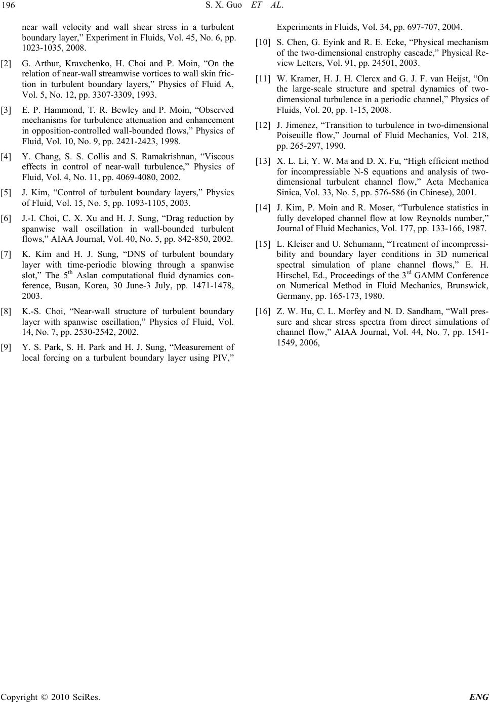

S. X. Guo ET AL. 196
near wall velocity and wall shear stress in a turbulent
boundary layer,” Experiment in Fluids, Vol. 45, No. 6, pp.
1023-1035, 2008.
[2] G. Arthur, Kravchenko, H. Choi and P. Moin, “On the
relation of near-wall streamwise vortices to wall skin fric-
tion in turbulent boundary layers,” Physics of Fluid A,
Vol. 5, No. 12, pp. 3307-3309, 1993.
[3] E. P. Hammond, T. R. Bewley and P. Moin, “Observed
mechanisms for turbulence attenuation and enhancement
in opposition-controlled wall-bounded flows,” Physics of
Fluid, Vol. 10, No. 9, pp. 2421-2423, 1998.
[4] Y. Chang, S. S. Collis and S. Ramakrishnan, “Viscous
effects in control of near-wall turbulence,” Physics of
Fluid, Vol. 4, No. 11, pp. 4069-4080, 2002.
[5] J. Kim, “Control of turbulent boundary layers,” Physics
of Fluid, Vol. 15, No. 5, pp. 1093-1105, 2003.
[6] J.-I. Choi, C. X. Xu and H. J. Sung, “Drag reduction by
spanwise wall oscillation in wall-bounded turbulent
flows,” AIAA Journal, Vol. 40, No. 5, pp. 842-850, 2002.
[7] K. Kim and H. J. Sung, “DNS of turbulent boundary
layer with time-periodic blowing through a spanwise
slot,” The 5th Aslan computational fluid dynamics con-
ference, Busan, Korea, 30 June-3 July, pp. 1471-1478,
2003.
[8] K.-S. Choi, “Near-wall structure of turbulent boundary
layer with spanwise oscillation,” Physics of Fluid, Vol.
14, No. 7, pp. 2530-2542, 2002.
[9] Y. S. Park, S. H. Park and H. J. Sung, “Measurement of
local forcing on a turbulent boundary layer using PIV,”
Experiments in Fluids, Vol. 34, pp. 697-707, 2004.
[10] S. Chen, G. Eyink and R. E. Ecke, “Physical mechanism
of the two-dimensional enstrophy cascade,” Physical Re-
view Letters, Vol. 91, pp. 24501, 2003.
[11] W. Kramer, H. J. H. Clercx and G. J. F. van Heijst, “On
the large-scale structure and spetral dynamics of two-
dimensional turbulence in a periodic channel,” Physics of
Fluids, Vol. 20, pp. 1-15, 2008.
[12] J. Jimenez, “Transition to turbulence in two-dimensional
Poiseuille flow,” Journal of Fluid Mechanics, Vol. 218,
pp. 265-297, 1990.
[13] X. L. Li, Y. W. Ma and D. X. Fu, “High efficient method
for incompressiable N-S equations and analysis of two-
dimensional turbulent channel flow,” Acta Mechanica
Sinica, Vol. 33, No. 5, pp. 576-586 (in Chinese), 2001.
[14] J. Kim, P. Moin and R. Moser, “Turbulence statistics in
fully developed channel flow at low Reynolds number,”
Journal of Fluid Mechanics, Vol. 177, pp. 133-166, 1987.
[15] L. Kleiser and U. Schumann, “Treatment of incompressi-
bility and boundary layer conditions in 3D numerical
spectral simulation of plane channel flows,” E. H.
Hirschel, Ed., Proceedings of the 3rd GAMM Conference
on Numerical Method in Fluid Mechanics, Brunswick,
Germany, pp. 165-173, 1980.
[16] Z. W. Hu, C. L. Morfey and N. D. Sandham, “Wall pres-
sure and shear stress spectra from direct simulations of
channel flow,” AIAA Journal, Vol. 44, No. 7, pp. 1541-
1549, 2006,