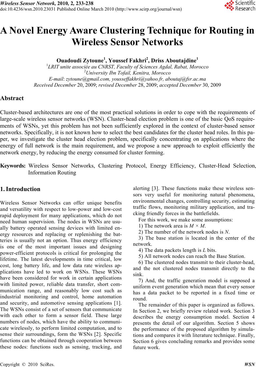Wireless Sensor Network, 2010, 2, 233-238
doi:10.4236/wsn.2010.23031 Published Online March 2010 (http://www.scirp.org/journal/wsn)
A Novel Energy Aware Clustering Technique for Routing in
Wireless Sensor Networks
Ouadoudi Zytoune1, Youssef Fakhri2, Driss Aboutajdine1
1LRIT unite associée au CNRST, Faculty of Sciences Agdal, Rabat, Morocco
2University Ibn Tofail, Kenitra, Morocco
Received December 20, 2009; revised December 28, 2009; accepted December 30, 2009
Abstract
Cluster-based architectures are one of the most practical solutions in order to cope with the requirements of
large-scale wireless sensor networks (WSN). Cluster-head election problem is one of the basic QoS require-
ments of WSNs, yet this problem has not been sufficiently explored in the context of cluster-based sensor
networks. Specifically, it is not known how to select the best candidates for the cluster head roles. In this pa-
per, we investigate the cluster head election problem, specifically concentrating on applications where the
energy of full network is the main requirement, and we propose a new approach to exploit efficiently the
network energy, by reducing the energy consumed for cluster forming.
Keywords: Wireless Sensor Networks, Clustering Protocol, Energy Efficiency, Cluster-Head Selection,
Information Routing
1. Introduction
Wireless Sensor Networks can offer unique benefits
and versatility with respect to low-power and low-cost
rapid deployment for many applications, which do not
need human supervision. The nodes in WSNs are usu-
ally battery operated sensing devices with limited en-
ergy resources and replacing or replenishing the bat-
teries is usually not an option. Thus energy efficiency
is one of the most important issues and designing
power-efficient protocols is critical for prolonging the
lifetime. The latest developments in time critical, low
cost, long battery life, and low data rate wireless ap-
plications have led to work on WSNs. These WSNs
have been considered for work in certain applications
with limited power, reliable data transfer, short com-
munication range, and reasonably low cost such as
industrial monitoring and control, home automation
and security, and automotive sensing applications [1].
The WSNs consist of a set of sensors that communicate
with each other to form a sensor field. These large
numbers of nodes, which have the ability to communi-
cate wirelessly, to perform limited computation, and to
sense their surroundings, form the WSNs [2]. Specific
functions can be obtained through cooperation between
these nodes: functions such as sensing, tracking, and
alerting [3]. These functions make these wireless sen-
sors very useful for monitoring natural phenomena,
environmental changes, controlling security, estimating
traffic flows, monitoring military application, and tra-
cking friendly forces in the battlefields.
For this work, we make some assumptions:
1) The network area is M × M.
2) The number of the network nodes is N.
3) The base station is located in the center of the
network.
4) The data packets length is L bits.
5) All network nodes can reach the Base Station.
6) The clustered nodes transmit to their cluster-head,
and the not clustered nodes transmit directly to the
sink.
7) And, the traffic generation model is supposed a
uniform event generation which mean that every sensor
has a data packet to be reported in a fixed time or
round.
The remainder of this paper is organized as follows.
In Section 2, we briefly review related work. Section 3
describes the energy consumption model. Section 4
presents the detail of our algorithm. Section 5 shows
the performance of the proposed algorithm by simula-
tions and compares it with literature technique. Finally,
Section 6 gives concluding remarks and provides some
future work.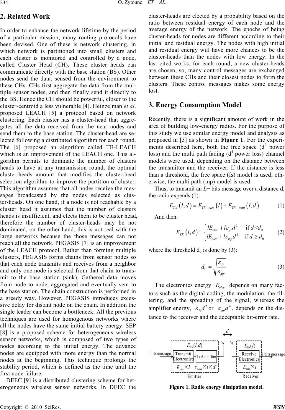

O. Zytoune ET AL. 234
2. Related Work
In order to enhance the network lifetime by the period
of a particular mission, many routing protocols have
been devised. One of these is network clustering, in
which network is partitioned into small clusters and
each cluster is monitored and controlled by a node,
called Cluster Head (CH). These cluster heads can
communicate directly with the base station (BS). Other
nodes send the data, sensed from the environment to
these CHs. CHs first aggregate the data from the mul-
tiple sensor nodes, and then finally send it directly to
the BS. Hence the CH should be powerful, closer to the
cluster-centroid a less vulnerable [4]. Heinzelman et al.
proposed LEACH [5] a protocol based on network
clustering. Each cluster has a cluster-head that aggre-
gates all the data received from the near nodes and
send them to the base station. The cluster-head are se-
lected following a distributed algorithm for each round.
The [6] proposed an algorithm called TB-LEACH
which is an improvement of the LEACH one. This al-
gorithm permits to dominate the number of clusters
heads to have at any transmission round, the optimal
cluster-heads amount that modifies the cluster-head
selection algorithm to improve the partition of cluster.
This algorithm assumes that all nodes receive the mes-
sages broadcasted by the nodes selected as clus-
ter-heads. On one hand, if a node is not reachable by a
cluster head it assumes that the number of clusters
heads is insufficient, and elects them to be cluster head,
therefore the number of cluster-heads may be not
dominated, on the other hand, this is not real with the
large networks because the those messages can not
reach all the network. PEGASIS [7] is an improvement
of the LEACH protocol. Rather than forming multiple
clusters, PEGASIS forms chains from sensor nodes so
that each node transmits and receives from a neighbor
and only one node is selected from that chain to trans-
mit to the base station (sink). Gathered data moves
from node to node, aggregated and eventually sent to
the base station. The chain construction is performed in
a greedy way. However, PEGASIS introduces exces-
sive delay for distant node on the chain. In addition the
single leader can become a bottleneck. All the previous
techniques are used for homogenous networks where
all the nodes have the same initial battery energy. SEP
[8] is a proposed scheme for heterogeneous wireless
sensor networks, which is composed of two types of
nodes according to the initial energy. The advance
nodes are equipped with more energy than the normal
nodes at the beginning. This technique prolongs the
stability period, which is defined as the time until the
first node failure.
DEEC [9] is a distributed clustering scheme for het-
erogeneous wireless sensor networks. In DEEC the
cluster-heads are elected by a probability based on the
ratio between residual energy of each node and the
average energy of the network. The epochs of being
cluster-heads for nodes are different according to their
initial and residual energy. The nodes with high initial
and residual energy will have more chances to be the
cluster-heads than the nodes with low energy. In the
last cited works, for each round, a new cluster-heads
are chosen, so, many control messages are exchanged
between these CHs and their closest nodes to form the
clusters. These control messages makes some energy
lost.
3. Energy Consumption Model
Recently, there is a significant amount of work in the
area of building low-energy radios. For the purpose of
this study we use similar energy model and analysis as
proposed in [5] as shown in Figure 1. For the experi-
ments described here, both the free space (d2 power
loss) and the multi path fading (d4 power loss) channel
models were used, depending on the distance between
the transmitter and the receiver. If the distance is less
than a threshold, the free space (fs) model is used; oth-
erwise, the multi path (mp) model is used.
Thus, to transmit an L− bits message over a distance d,
the radio expends (1):






,,
TXTX elecTX amp
Eld ElEld

 (1)
And then:

2
0
4
0
if <
,if
elec fs
TX
elec mp
lEldd d
Eld lEldd d






 (2)
where the threshold d0 is done by (3):
0
fs
mp
d


 (3)
The electronics energy depends on many fac-
tors such as the digital coding, the modulation, the fil-
tering, and the spreading of the signal, whereas the
amplifier energy, or , depends on the dis-
tance to the receiver and the acceptable bit-error rate.
elec
E
mp d

2
fs d

4
Figure 1. Radio energy dissipation model.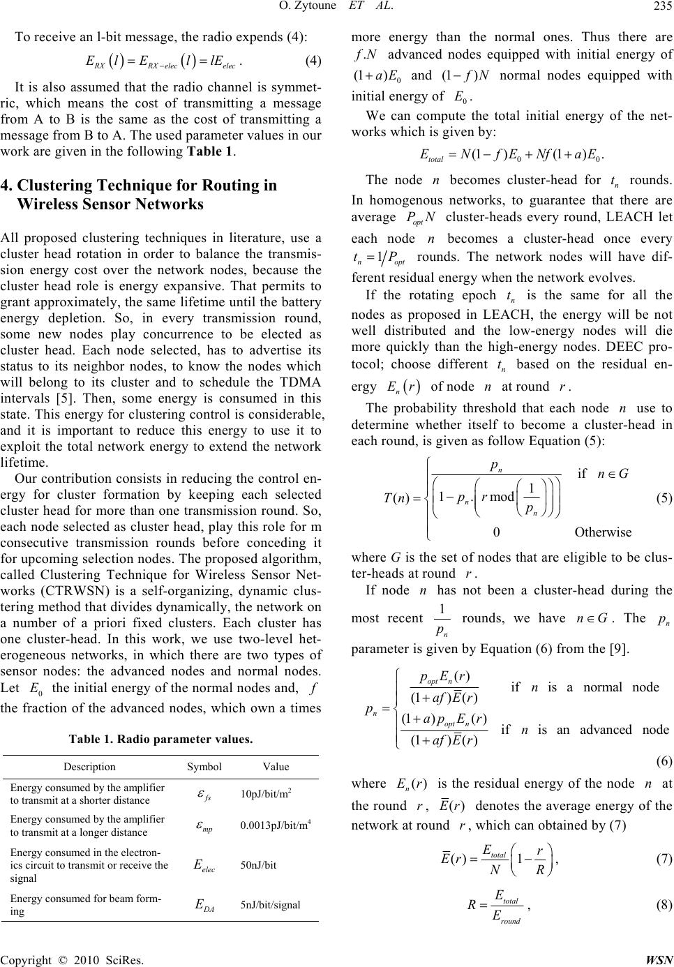

O. Zytoune ET AL.235
To receive an l-bit message, the radio expends (4):
 
R
XRXelec
ElE llE


elec
. (4)
It is also assumed that the radio channel is symmet-
ric, which means the cost of transmitting a message
from A to B is the same as the cost of transmitting a
message from B to A. The used parameter values in our
work are given in the following Table 1.
4. Clustering Technique for Routing in
Wireless Sensor Networks
All proposed clustering techniques in literature, use a
cluster head rotation in order to balance the transmis-
sion energy cost over the network nodes, because the
cluster head role is energy expansive. That permits to
grant approximately, the same lifetime until the battery
energy depletion. So, in every transmission round,
some new nodes play concurrence to be elected as
cluster head. Each node selected, has to advertise its
status to its neighbor nodes, to know the nodes which
will belong to its cluster and to schedule the TDMA
intervals [5]. Then, some energy is consumed in this
state. This energy for clustering control is considerable,
and it is important to reduce this energy to use it to
exploit the total network energy to extend the network
lifetime.
Our contribution consists in reducing the control en-
ergy for cluster formation by keeping each selected
cluster head for more than one transmission round. So,
each node selected as cluster head, play this role for m
consecutive transmission rounds before conceding it
for upcoming selection nodes. The proposed algorithm,
called Clustering Technique for Wireless Sensor Net-
works (CTRWSN) is a self-organizing, dynamic clus-
tering method that divides dynamically, the network on
a number of a priori fixed clusters. Each cluster has
one cluster-head. In this work, we use two-level het-
erogeneous networks, in which there are two types of
sensor nodes: the advanced nodes and normal nodes.
Let the initial energy of the normal nodes and,
0
E
f
the fraction of the advanced nodes, which own a times
Table 1. Radio parameter values.
Description Symbol Value
Energy consumed by the amplifier
to transmit at a shorter distance fs

10pJ/bit/m2
Energy consumed by the amplifier
to transmit at a longer distance mp

0.0013pJ/bit/m4
Energy consumed in the electron-
ics circuit to transmit or receive the
signal elec
E 50nJ/bit
Energy consumed for beam form-
ing
D
A
E 5nJ/bit/signal
more energy than the normal ones. Thus there are
.
f
N
(1
advanced nodes equipped with initial energy of
0
)aE

and (1 )
f
N

normal nodes equipped with
initial energy of .
0
E
We can compute the total initial energy of the net-
works which is given by:
00
(1)(1) .
total
ENfENfaE


The node becomes cluster-head for rounds.
In homogenous networks, to guarantee that there are
average cluster-heads every round, LEACH let
each node becomes a cluster-head once every
n
N
n
n
t
opt
P
1
nopt
Pt

rounds. The network nodes will have dif-
ferent residual energy when the network evolves.
If the rotating epoch is the same for all the
nodes as proposed in LEACH, the energy will be not
well distributed and the low-energy nodes will die
more quickly than the high-energy nodes. DEEC pro-
tocol; choose different t based on the residual en-
ergy
n
t
n


n
Er of node at round r. n
The probability threshold that each node use to
determine whether itself to become a cluster-head in
each round, is given as follow Equation (5):
n
if
1
1.mod
()
0Othe
n
n
n
pnG
pr
Tn p







 



 

rwise
(5)
where G is the set of nodes that are eligible to be clus-
ter-heads at round . r
If node has not been a cluster-head during the
most recent
n
1
n
p rounds, we have . The
parameter is given by Equation (6) from the [9].
nGn p
() ifis anormal node
(1)( )
(1)( )ifis anadvanced node
(1)( )
opt n
n
opt n
pErn
afE r
papE rn
afE r







(6)
where is the residual energy of the node at
the round ,
()
n
Er
r
n
()Er denotes the average energy of the
network at round , which can obtained by (7) r
() 1
total
Er
Er NR






, (7)
total
round
E
RE , (8)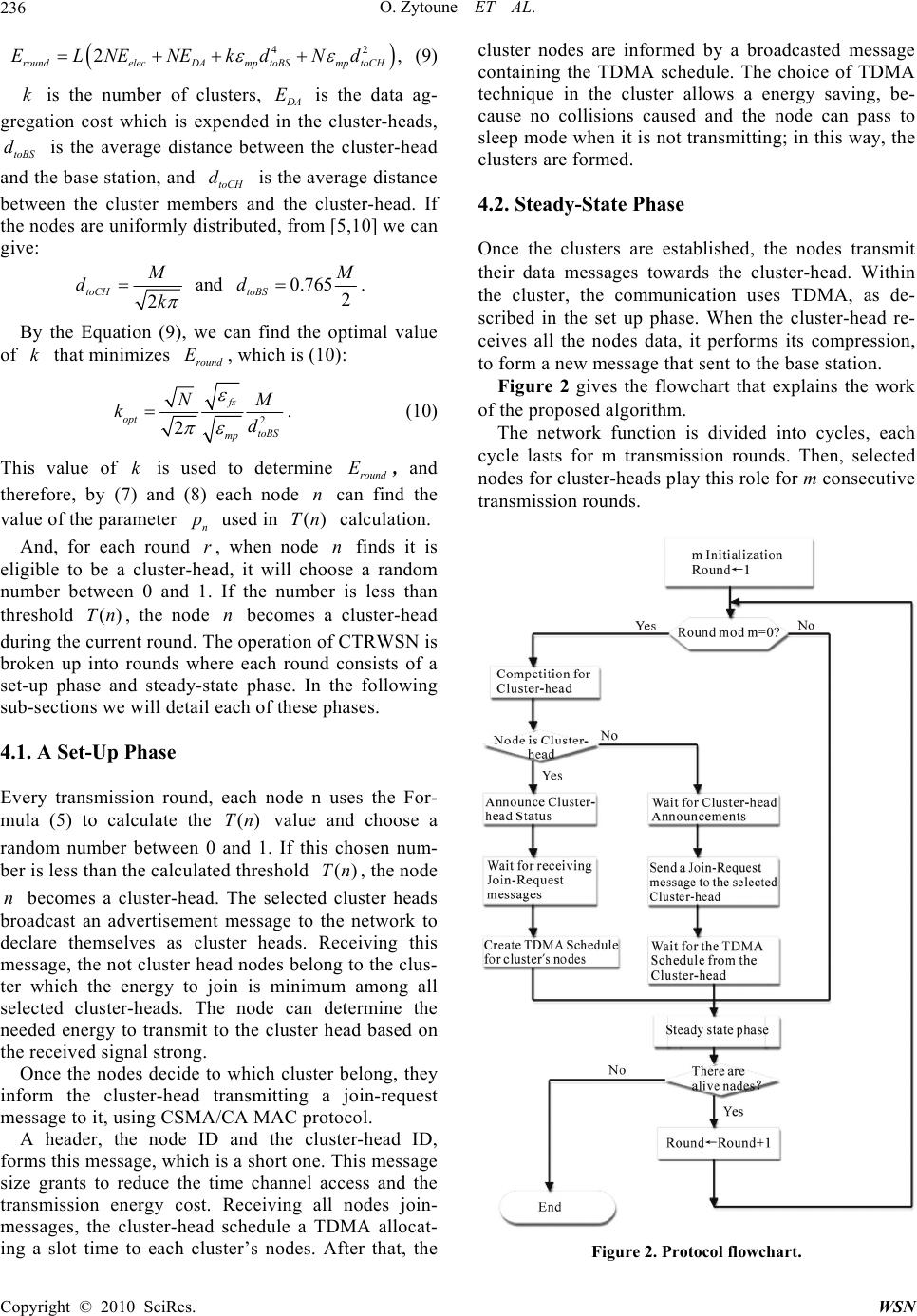

O. Zytoune ET AL. 236

,

42
2
roundelecDAmp toBSmp toCH
EL NENEkdNd   (9)
k is the number of clusters,
D
A
E is the data ag-
gregation cost which is expended in the cluster-heads,
is the average distance between the cluster-head
and the base station, and is the average distance
between the cluster members and the cluster-head. If
the nodes are uniformly distributed, from [5,10] we can
give:
toBS
d
toCH
d
and0.765 2
2
toCH toBS
M
M
dd
k

.
By the Equation (9), we can find the optimal value
of that minimizes , which is (10):
kround
E
2
2
fs
opt
toBS
mp
N
kd


M . (10)
This value of is used to determine , and
therefore, by (7) and (8) each node can find the
value of the parameter used in calculation.
kround E
n
()Tn
n
p
And, for each round , when node finds it is
eligible to be a cluster-head, it will choose a random
number between 0 and 1. If the number is less than
threshold , the node becomes a cluster-head
during the current round. The operation of CTRWSN is
broken up into rounds where each round consists of a
set-up phase and steady-state phase. In the following
sub-sections we will detail each of these phases.
rn
()Tn n
4.1. A Set-Up Phase
Every transmission round, each node n uses the For-
mula (5) to calculate the value and choose a
random number between 0 and 1. If this chosen num-
ber is less than the calculated threshold , the node
becomes a cluster-head. The selected cluster heads
broadcast an advertisement message to the network to
declare themselves as cluster heads. Receiving this
message, the not cluster head nodes belong to the clus-
ter which the energy to join is minimum among all
selected cluster-heads. The node can determine the
needed energy to transmit to the cluster head based on
the received signal strong.
()Tn
()Tn
n
Once the nodes decide to which cluster belong, they
inform the cluster-head transmitting a join-request
message to it, using CSMA/CA MAC protocol.
A header, the node ID and the cluster-head ID,
forms this message, which is a short one. This message
size grants to reduce the time channel access and the
transmission energy cost. Receiving all nodes join-
messages, the cluster-head schedule a TDMA allocat-
ing a slot time to each cluster’s nodes. After that, the
cluster nodes are informed by a broadcasted message
containing the TDMA schedule. The choice of TDMA
technique in the cluster allows a energy saving, be-
cause no collisions caused and the node can pass to
sleep mode when it is not transmitting; in this way, the
clusters are formed.
4.2. Steady-State Phase
Once the clusters are established, the nodes transmit
their data messages towards the cluster-head. Within
the cluster, the communication uses TDMA, as de-
scribed in the set up phase. When the cluster-head re-
ceives all the nodes data, it performs its compression,
to form a new message that sent to the base station.
Figure 2 gives the flowchart that explains the work
of the proposed algorithm.
The network function is divided into cycles, each
cycle lasts for m transmission rounds. Then, selected
nodes for cluster-heads play this role for m consecutive
transmission rounds.
Figure 2. Protocol flowchart.

O. Zytoune ET AL.237
It is so difficult to determine analytically the pa-
rameter m, because the nodes deployment is random
and the cluster-heads position is also stochastic, then
we determine this optimal value based on simulation.
5. Simulation and Results
The simulation parameters values used in our work are
given in the Table 2.
For the simulation bellow, we fix f = 0.2 and a = 3.
Figure 3 represents the DEEC energy consumed in the
network for the clusters forming for every transmission
round. This energy is expended by the messages ex-
changed between the cluster-heads and its belonging
nodes to form the clusters. As we can see, a lot of the
network energy is lost to control the clusters formations.
The total of this energy is evaluated as 33.3824J which
is 41.73% of the total network energy, and in average
0.0057J per round.
To find the optimal value of the parameter m, we do
simulation by varying it. Figure 4 gives the relative
network lifetime. As depicted in this figure, the relative
network lifetime becomes approximately constant
when the parameter m is greater than 10. This lifetime
is maximal when the cluster-head duration m is equal
to 32; each node selected as cluster-head, plays this
role for m consecutive transmission rounds that permits
to economize the energy consumed by the clus-
ter-heads to form their clusters, because the number of
control messages is reduced. As we can see in the fig-
ure, if the cluster-head period duration becomes longer
than a threshold, even if the network control energy is
reduced, oppositely, the network lifetime decreases
slightly. The reason of that is the unbalancing of the
cluster-heads energy load over the network nodes. So,
some nodes are highly solicited when they belong to a
cluster. Continuing to belong to the same cluster, some
unlucky nodes have to transmit for larger distance, and
then there energy drains quickly. We can see in Figure
5 the energy for forming the clusters in the CTRWSN.
Figure 6 gives the network lifetime of the proposed pro-
tocol compared to DEEC one. The first node dies in the
718th round but in CTRWSN it occurs in the 1271st
Table 2. Simulation parameter values.
Description Symbol Value
Network dimension M 100m
Number of network nodes N 100
Data packet length L 4000bits
Control packet length Lcrt 200bits
Optimal probability popt 0.1
Advanced Nodes percentage f Variable
Fraction of advanced nodes energy
to normal nodes a Variable
Figure 3. Total network energy for Clusters forming in DEEC.
Figure 4. Relative network lifetime.
Figure 5. Total network energy for clusters forming in
CTRWSN.
round, which means that the stable region is extended by
up to 77%. The half network nodes die in DEEC at the
832nd round and in CTRWSN it happens in the 1898th
round and the last node die in the 5865th in DEEC, and
9494th round in CTRWSN, which is approximately 62%
longer than DEEC.
Figure 7 gives the network remaining energy. The av-
erage network remaining energy in DEEC is 10.2149J/round
and in CTRWSN is 13.9502/round that means that the
CTRWSN consumes little energy compared to DEEC,
which helps to extend the network lifetime for many ex-
tra-rounds.

O. Zytoune ET AL. 238
6. Conclusions and Future Works
Figures 8(a) and 8(b) gives the network lifetime de-
fined until the first node dies when a and f are varying.
This figure shows that the proposed technique pro-
vides best results when the network parameters change.
In this paper, we have proposed a clustering based rout-
ing protocol for heterogeneous WSNs, which is entirely
distributed. We have interested in reducing the number
of control message, and so, the protocol overhead.
Through the simulation, we demonstrate that the pro-
posed algorithm allows a large stable network lifetime
compared to the most known clustering algorithms in this
area. As future work, we will reconsider the probability of
becoming cluster-head, to extend yet the network lifetime.
7. Acknowledgements
Figure 6. Network lifetime comparison.
This work was supported by the Hassan II Académie des
Sciences et Techniques.
8. References
[1] F. Akyidiz, W. Su, Y. Sankarasubramaniam, and E. Cay-
irci, “Wireless sensor network: A survey,” Computer
Networks, Vol. 38, No. 4, pp. 393–422, 2002.
[2] K. Romer, O. Kastin, and F. Mattern, “Middleware chal-
lenges for wireless sensor networks,” ACM SIGMOBILE
Mobile Computing and Communications Review, Vol. 6,
No. 4, pp. 59–61, 2002.
Figure 7. Network remaining energy comparison.
[3] R. Shorey, A. Ananda, and W. T. Ooi, “Mobile, wireless,
and sensor networks,” 1st edition, IEEE Press, John
Wiley & Sons, 2006.
[4] Z. Khalid, G. Ahmed, N. M. Khan, and P. Vigneras, “A
real-time energy-aware routing strategy for wireless sen-
sor networks,” Asia-Pacific Conference on Communica-
tions, Bangkok, Thailand, pp. 381–384, 2007.
[5] W. R. Heinzelman, A. P. Chandrakasan, and H. Bala-
krishnan, “An application-specific protocol architecture for
wireless microsensor networks,” IEEE Transactions on
Wireless Communications, Vol. 1, No. 4, pp. 660–670, 2002.
[6] J. Hu, Y. Jin, and L. Dou, “A time-based cluster-head
selection algorithm for LEACH”, Proceeding of IEEE
Symposium on Computers and Communications, Marra-
kech, Morocco, 6–9 July 2008.
(a)
[7] S. Lindsey and C. S. Raghavendra, “PEGASIS: Power
efficient gathering in sensor information systems,” Pro-
ceedings of the IEEE Aerospace Conference, Big Sky,
Montana, March 2002.
[8] G. Smaragdakis, I. Matta, and A. Bestavros, “SEP: A
stable election protocol for clustered heterogeneous wireless
sensor networks,” Second International Workshop on Sensor
and Actor Network Protocols and Applications, 2004.
[9] L. Qing, Q. X. Zhu, and M. W. Wang, “Design of a dis-
tributed energy—efficient clustering algorithm for hetero-
geneous wireless sensor networks,” Computer Communi-
cation, Elsevier, Vol. 29, No. 12, pp. 2230–2237, 2006.
[10] S. Bandyopadhyay and E. J. Coyle, “An energy efficient
hierarchical clustering algorithm for wireless sensor net-
works,” Proceeding of International Conference on Com-
puter Communication, Vol. 3, pp. 1713–1723, April 2003.
(b)
Figure 8. Network lifetime until the first node dies. (a) f = 0.2 and
a varying from 0.5 to 5; (b) a = 3 and f varying from 0.1 to 0.9.