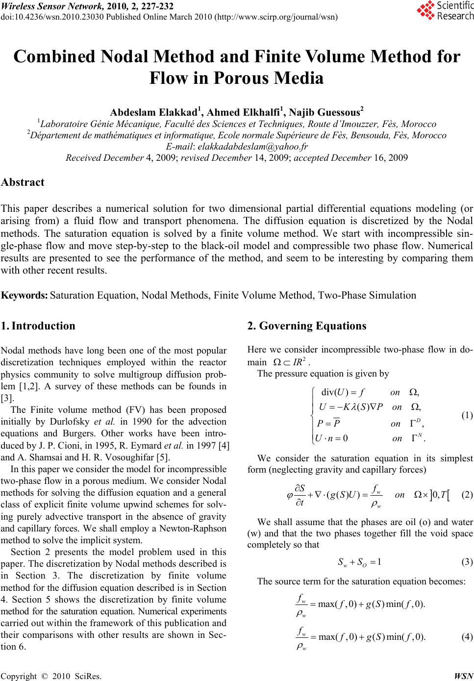Wireless Sensor Network, 2010, 2, 227-232
doi:10.4236/wsn.2010.23030 Published Online March 2010 (http://www.scirp.org/journal/wsn)
Combined Nodal Method and Finite Volume Method for
Flow in Porous Media
Abdeslam Elakkad1, Ahmed Elkhalfi1, Najib Guessous2
1Laboratoire Génie Mécanique, Faculté des Sciences et Techniques, Route d’Imouzzer, Fès, Morocco
2Département de mathématiques et informatique, Ecole normale Supérieure de Fès, Bensouda, Fès, Morocco
Received December 4, 2009; revised December 14, 2009; accepted December 16, 2009
Abstract
This paper describes a numerical solution for two dimensional partial differential equations modeling (or
arising from) a fluid flow and transport phenomena. The diffusion equation is discretized by the Nodal
methods. The saturation equation is solved by a finite volume method. We start with incompressible sin-
gle-phase flow and move step-by-step to the black-oil model and compressible two phase flow. Numerical
results are presented to see the performance of the method, and seem to be interesting by comparing them
with other recent results.
Keywords: Saturation Equation, Nodal Methods, Finite Volume Method, Two-Phase Simulation
1. Introduction
Nodal methods have long been one of the most popular
discretization techniques employed within the reactor
physics community to solve multigroup diffusion prob-
lem [1,2]. A survey of these methods can be founds in
[3].
The Finite volume method (FV) has been proposed
initially by Durlofsky et al. in 1990 for the advection
equations and Burgers. Other works have been intro-
duced by J. P. Cioni, in 1995, R. Eymard et al. in 1997 [4]
and A. Shamsai and H. R. Vosoughifar [5].
In this paper we consider the model for incompressible
two-phase flow in a porous medium. We consider Nodal
methods for solving the diffusion equation and a general
class of explicit finite volume upwind schemes for solv-
ing purely advective transport in the absence of gravity
and capillary forces. We shall employ a Newton-Raphson
method to solve the implicit system.
Section 2 presents the model problem used in this
paper. The discretization by Nodal methods described is
in Section 3. The discretization by finite volume
method for the diffusion equation described is in Section
4. Section 5 shows the discretization by finite volume
method for the saturation equation. Numerical experiments
carried out within the framework of this publication and
their comparisons with other results are shown in Sec-
tion 6.
2. Governing Equations
Here we consider incompressible two-phase flow in do-
main 2
IR

.
The pressure equation is given by
div( ),
() ,
,
0.
D
N
Uf on
UKSPon
PP on
Un on






 









(1)
We consider the saturation equation in its simplest
form (neglecting gravity and capillary forces)

(() )0,
w
w
f S

g
SUon T
t

 
 (2)
We shall assume that the phases are oil (o) and water
(w) and that the two phases together fill the void space
completely so that
1


wO
SS (3)
The source term for the saturation equation becomes:
max( ,0)()min(,0).


w
w
ffgS f
max(, 0)() min(,0).


w
w
ffgS f
(4)

A. Elakkad ET AL. 228
where
2
22
() (1 ) 
S
gS SS
To close the model, we must also supply expressions
for the saturation-dependent quantities. Here we use
simple analytical expressions:
22
0
0
()(1 )
(), (),1
wc
w
worwc
SS
SS
SSS
SS







K is the permeability,

is the Rock porosity, 0

and

w
wc
S
Viscosities, is the irreducible oil satura-
tion, is the connate water saturation, and the total
mobility is given by
or
S
0

 
w.
3. Discretization with Nodal Methods
The discretizations which follow assume that

is a
rectangular domain and employ an tensor prod-
uct mesh having cells
LM
,11 1
22 2
(, )()
 
 
ij ii j
xxy y
1
2
,

j
.
It is convenient to denote the mesh spacing by
1
22

 
iii 1
x
xx
and 11
22


 
jjj
yy y
.
Common to all nodal discretizations is the choice of
cell-and edge-based unknowns. Generally, these are tak-
en to be moments up to some specified order; hence in
the lowest-order case simple averages are employed.
Specifically, the cell-based unknowns are averages de-
fined by
11
22
11
22
,
1(, )


 
ij
ij
xy
ij xy
ij
PPxy dxdy
xy (5)
while the edge-based scalar unknowns, namely, edge
averages of the scalar flux, are given by
1
2
1
2
11
,
22
1
(),() (,)




j
j
y
jj y
ij ij
PPxPxPxyd
yy (6)
with the analogous definitions of 1
,2 ij
P and .
Similarly, the edge-averaged currents are written as
()
i
Py

1
2
1
1
2
1,
2
1
lim( ),( )( 












j
j
i
y
jj y
ij xx j
UUxUx Kydy
yx
2
, )Px
while 1
,2


ij
U is defined analogously.
All lowest-order members of the nodal method family,
such as the nodal expansion methods (NEM) [6], the
nodal integration method (NIM) [7], the nodal Green's
function method (NGFM) [8] and the coarse mesh ex-
pansion methods [9] yield equivalent discretization of (1).
We have chosen to present a brief discussion of the NIM.
The first step in the NIM discretization consists of posing
the cell-based trans-verse integrated ODEs which govern
and . To this end we assume that a ho-
mogenized diffusion coefficient
()
j
Px ()
i
Py
()

ij
K is defined on
each cell, and transverse integrate (1) to obtain

11 1
22 2
1
()()() (),,


 

  

 
 



jj
ij jj i
j
KPx UxUxfxxxx
xx y1
2


i

11 1
22 2
1
()()()(),,


 
 
 

 
 
 

ii
ij ii j
i
KPyUyUyfyyyx
yy x1
2


j
where 1
2
()


j
Ux and 1
2


i
U are one-sided limits of the
normal currents along the edges of the cell, and
j
f
is
defined in analogy with the transverse averaged un-
knowns.
Thus, we have reduced the discretization of the PDE
given in (1) to that of two ODEs that are coupled through
pseudo source terms. The definition of the edge averages
(6) naturally yields Dirichlet boundary conditions for each
cell. Moreover, for lowest-order or constant-constant NIM
the pseudo source term (i.e. 1
2
()


j
Ux and 1
2
()


i
Uy) are
assumed to be constant along their respective cell edges.
We assume that the source (, )
f
xy is constant over
each cell.
With expressions for and in hand we
construct the discretization. First, note that two inde-
pendent definitions of the cell average are possible:
()
j
Px ()
i
Py
11
22
11
22
,
11
() ()





ij
ij
xy
ij ji
xy
ij
PPxdxP
xy
ydy
Yielding 2LM equations, e.g.
 1
2
21
,11 1
, ,
,, ,
22 2
11
()
212



 




 




i
ij ij
ij ij
ij ijij
j
x
PPPKUU f
y,
.
Furthermore, under the assumption of an homogenized
diffusion coefficient and utilizing ()

 UKSP we
obtain expressions for 11
,

,
22
,


ij ij
UU, on each cell, e.g.


,
111 11
,,, ,,
222 22
11
() ()
2


 


 




ij
ij
ijij ijijij
iij
K
UPPUU
xxy
,

f
Although these compriseations per cell, only
th
for equ
ree of them are linearly independent, as the same bal-
ance equation arises from both 11

UU and
,,
22
 ij ij
11
,,
2
.



ij ij
UU
2

Imposing continuity of
J
n yields an
equation for each interior edge (i.e. (L-1)M + L(M-1)
M discretization is
co
equations) while the boundary conditions give rise to 2L
+ 2M discrete boundary equations. Thus we have 7LM +
L + M equations as many unknowns.
Although the constant-constant NI
mplete at this point, it is seldom used in this form.
Typically in the literature one proceeds by eliminating

A. Elakkad ET AL.229
the edge currents 11 ,

UU, followed by the trivial
nearest neighbor hexagonally pled stencils that gov-
ern the edge-based fluxes
,,
22
 ij ij
elimination of the averages to obtain the 7-point
,ij
P
cou
1
P:
2
ij
 


11 31
,1,
,, ,,
1
22 22
,
11 11
22 ,,,,
22 22
1
1,
31 1
22 ,,1,
122 2
3
3




 

 




  
 
 
   

 
 
 

 

 




jj
iji j
ij ijij ij
ii
ij
ij
ij ij ijij
ij
ij
ij
ij ij iji
ij
yy
KPPK PP
xx
Kxy
PPPP
xy
Kxy
PPP P
xy



1
1, 2
33
1
,1,
222 2
1
11
22









 


j
iji j
iji j
iji j
xyx y
ff
xyx y


With the y-oriented rotateanalogue at d 1
,2
ij
P.
4. Finite Volume Method for the Diffusion
In e method for (1) one introduces a family
f control volumes (typically the given mesh) and im-
Equation
a finite volum
o
poses mass conservation locally for each control volume
E: .

 

EE
K
P ndsfdx, where n is the outward unit
norm tered finite volume method,
whi a pressure stencil for each
cell i E,

al on E. The cell-cen
ch may be expressed as
,
i ij ijE
j
TP Pfdx (7)
where j loops over all cells neighboring
issibilities
cell i E. The
transm ij T are associated with cell interfaces,
and the expressio


ij ij
TPP is a discrete form of
., 


ij
ij
EE
n
K
Pn ds is the unit normal on
ting into.
j
EThus,
where ij
n
 
ij ij
EE poin



ij ij
TPP
al flux across estimates the tot


rb
ij
itra
EE. Th
is clearly symmetric, and a solution is, as for the con-
tinuous problem, defined up tory constant. The
system is made positive definite and symmetry is pre-
served, by forcing 10P, for instance. That is, by add-
ing a positive constant to the first diagonal of the matrix

e sm (7)yste
an a

ik
A
a,
where
,
.





ij
j
ik
ik
Tifki
a
Tifki
(8)
The matrix A is sparse, consisting of a tridiagonal part
corresponding to the x-derivative, and t
bands corresponding to the y-derivatives.
(9)
where
wo off-diagonal
5. Finite Volume Method for the Saturation
Equation
For the saturation Equation (2), we use a finite volume
scheme on the form
   
1max, 0()min, 0

  




nntm m
iixiij i i
ijij
SSfgSUgS f







t
xi
ii
t, i

is the porosity in

i, i
f
denotes the source term,

t
er
is the time step, and
-average of the w
k
i
S is
the cellatsaturation at time

k
t, t

1,

i
k
ik
i
SSxtdx.

By specifying for time level m in the evaluation in the
fractional flow functions, we obtain either an explicit (m
= n) or implicit (m = n + 1) scheme. Here is the total
flu
ij
U
x (for oil and water) over the edge ij between two
adjacent cells

i and

j
, and ij
g
is the fractional
flow function at

ij
) 0,
() 


wi
gS ifU
gS (10)
( .
(). 0.


ij
wij
wj ij
n
gS ifUn
The explicit solver is obtained by using m = n in (9).
Explicit schemes are only stable provided
step
that the time

t satisfies a CFL condition. For the homogene-
ous transport equation (with 0f), the CFL condition
for the first-order upwind scheme reads

 
(0,1)
max'() max21 


t
x
ijwc or
i
Si
j
g
SUSS
(11)
For the inhomogeneous equation, we can derive a sta-
bility condition on

t using a more heuristic arg
Physically, we require that
ument.
11 

n
wc ior
SS S.
This implies that the discretization parameters

i
and

t must satisfy the following dynamic conditions:




max, 0()min, 01 


  




ntn n
i xiijii
jij
SfgSUgS f
(12)
wc or
i
S S
The interface fluxes satisfy the following mass
balance property:
ij
U

A. Elakkad ET AL. 230






max,0min,0min(,0)max ,0
.
 


in
iiij i
jj
out
i
UfUfU
U
Thus, since 0()1gS it follows that
ij
where and are array vectors that contain the
average pressure in each fine eleme
solution and reference finite volume solution, respec-
tively).
e
Pref P
nt (Nodal Methods
We masure velocity solution errors using the follow-
ing measure:


() max
ninn n
ii
gS U,0 ()()min(,0)
(1())
 

 iij ii
jij
nin
ii
fgS UgSf
gS U
22

ref ref
Then the general saturation dependent stability condi-
tio if the foll is satisfied: n holds in owing inequality
i

()01 ()
max ,1
1







nn
tin
ii
xi
nn
i
iwcori
gSgS U
SSS S (13)
Finally to remove the saturation dependence from (13),
w
er
e invoke the mean value theorem and deduce that (13)
holds whenev
 
01
max '



 i
in
iS
tUgS
In this section we illustrate the performance of the Nodal
methods. We restrict to quarter-five spot pr
dimensions with uniform rectangular grids [10,11]. We
ompare the solutions obtained using Nodal Methods
lution obtained using a
(14)
6. Numerical Simulations
oblems in two
c
with the reference fine scale so
two point finite volume method.
We compute a mean pressure error in the following
manner:

2
2



ref
ref
PP
P
P
(15)

22
 
xx yy
ref ref
U
UU
(16)
xx
UU UU
x
U and are vectors containing the average veloci-
ties in the x-and y-directions, respectively,
y
U
. and is
the Euclidean norm.
T ss
um
tio
. The reservoir is
he preure equation is discretized by the Nodal vol-
e method (FV). We use an Explicit and Implicit up-
wind finite volume discretization for the saturan Equa-
tion (2).
Example: Here, we present a simulator for incom-
pressible and immiscible Two-Phase flow system. We
first want to look at the so called the quarter-five spot
problems




0,1 0,1 
pure oil. To pro
with a unit
injection well placed at (0; 0) and a production well with
unit production rate placed at (1; 1). Let us revisit the
quarter-five spot problems, but now assume that the res-
ervoir is initially filled withduce the oil
in the upper-right corner, we inject water in the lower left.
We assume unit porosity, unit viscosities for both phases,
and set 0


or wc
SS . We impose no-flow boundary
conditions on

.
We obtain a similar result with J. E. Aarnes et al. [10].
The water saturation is increasing monotonically toward
the injectohat more oil is gradually displaced
as more water is injected,
r, meaning t
and the pressure fields are
symmetric.
Figuret 1. The left plot shows pressure contours for a homogeneous quarter-five spot obtained using Nodal Methods and the
right plot shows pressure contours for a homogeneous quarter-five spot with the reference solution obtained by J. E. Aarnes
et al. [10], with a 20 × 20 square grid.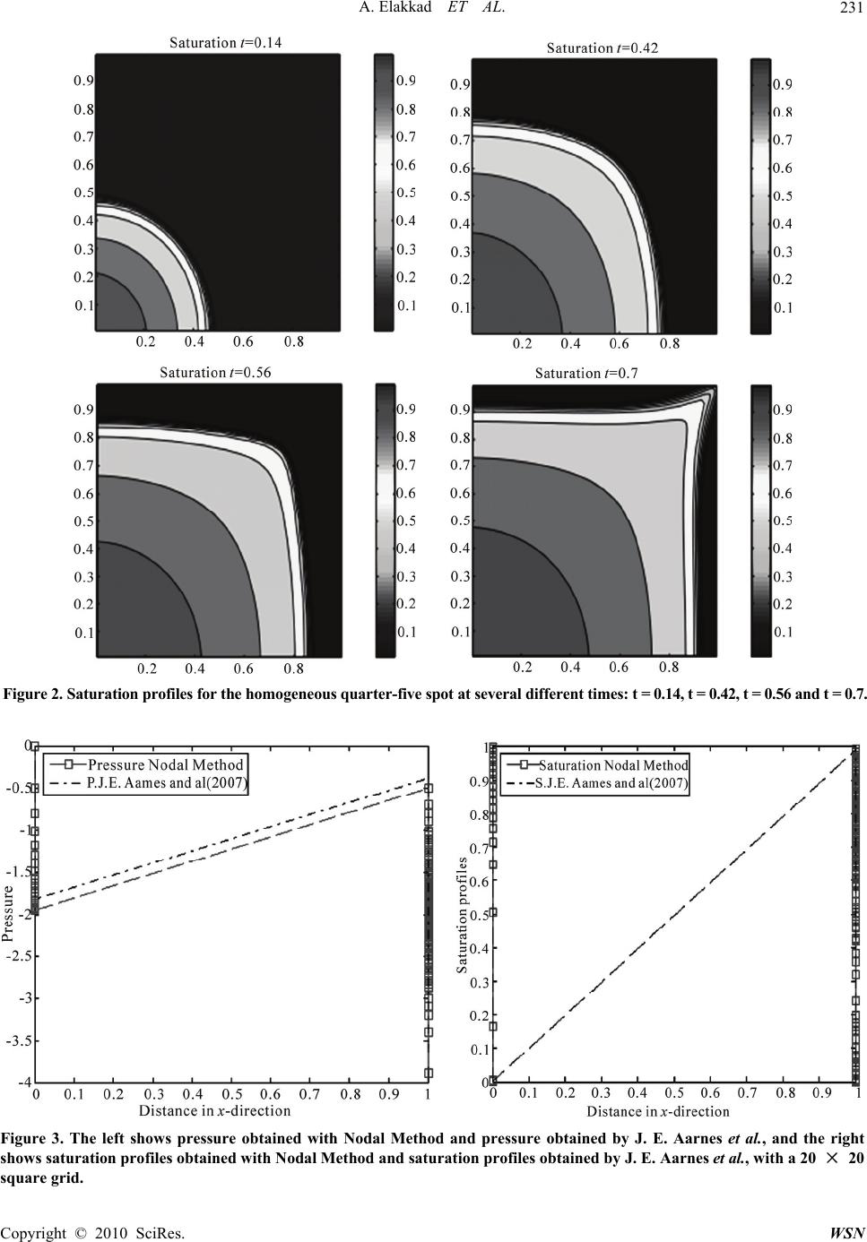

A. Elakkad ET AL.231
Figure 2. Saturation profiles for the homogeneous quarter-fiv at several different times: t = 0.14, t = 0.42, t = 0.56nd t = 0.7. e spot a
Figure 3. The left shows pressure obtained with Nodal Method and pressure obtained by J. E. Aarnes et al., and the right
shows saturation profiles obtained with Nodal Method and saturation profiles obtained by J. E. Aarnes et al., with a 20 × 20
square grid.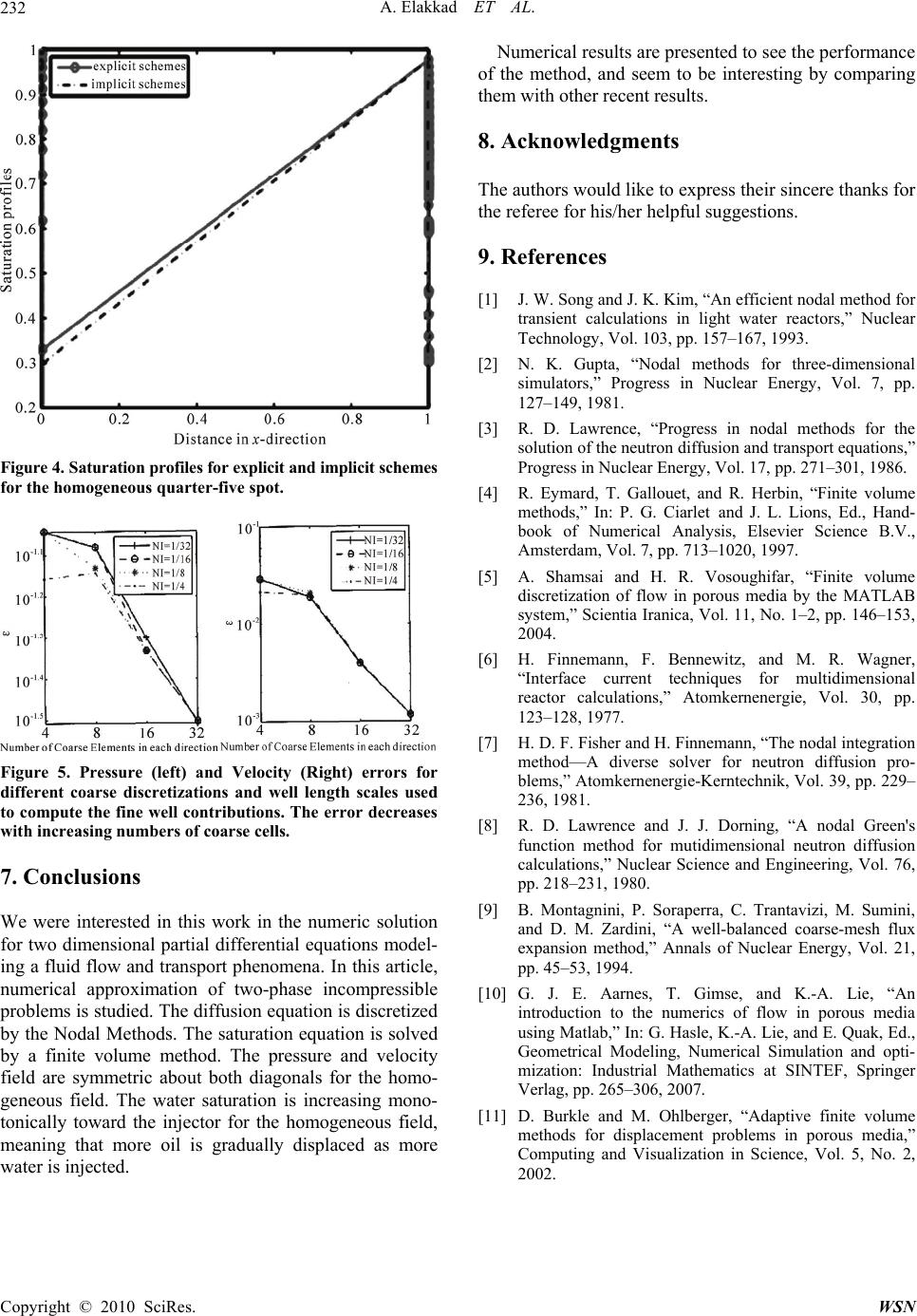

A. Elakkad ET AL. 232
Figure 4. Saturation profiles for explicit and implicit schemes
for the homogeneous quarter-five spot.
Figure 5. Pressure (left) and Velocity (Right) errors for
different coarse discretizations and well length scales used
to compute the fine well contributions. The error decreases
with increasing numbers of coarse cells.
7. Conclusions
We were interested in this work in the numeric solutio
pressible
problems is studied. The diffusion equation is discretized
by the Nodal Methods. The saturation equation is solved
by a finite volume method. The pressure and velocity
field are symmetric about both diagonals for the homo-
geneous field. The water saturation is increasing mono-
tonically toward the injector for the homogeneous field,
meaning that more oil is gradually displaced as more
water is injected.
Numerical results are presented to see the performance
of the method, and seem to be interesting by comparing
them with other recent results.
8. Acknowledgments
The authors would like to express their sincere thanks for
the referee for his/her helpful suggestions.
9. References
[1] J. W. Song and J. K. Kim, “An efficient nodal method for
transient calculations in light water reactors,” Nuclear
Technology, Vol. 103, pp. 157–167, 1993.
[2] N. K. Gupta, “Nodal methods for three-dimensional
simulators,” Progress in Nuclear Energy, Vol. 7, pp.
127–149, 1981.
R. D. Lawrence, “Progress in nodal methods for the
solution of the neutron diffusion and transport equations,
methods,” In: P. G. Ciarlet and J. L. Lions, Ed., Hand-
book of Numerical Analysis, Elsevier Science B.V.,
. 1–2, pp. 146–153,
F. Bennewitz, and M. R. Wagner,
“Interface current techniques for multidimensional
thod,” Annals of Nuclear Energy, Vol. 21,
pp. 45–53, 1994.
A. Lie, and E. Quak, Ed.,
Geometrical Modeling, Numerical Simulation and opti-
thematics at SINTEF, Springer
7.
Vol. 5, No. 2,
[3]
”
Progress in Nuclear Energy, Vol. 17, pp. 271–301, 1986.
[4] R. Eymard, T. Gallouet, and R. Herbin, “Finite volume
Amsterdam, Vol. 7, pp. 713–1020, 1997.
[5] A. Shamsai and H. R. Vosoughifar, “Finite volume
discretization of flow in porous media by the MATLAB
system,” Scientia Iranica, Vol. 11, No
2004.
[6] H. Finnemann,
reactor calculations,” Atomkernenergie, Vol. 30, pp.
123–128, 1977.
[7] H. D. F. Fisher and H. Finnemann, “The nodal integration
method—A diverse solver for neutron diffusion pro-
blems,” Atomkernenergie-Kerntechnik, Vol. 39, pp. 229–
236, 1981.
[8] R. D. Lawrence and J. J. Dorning, “A nodal Green's
function method for mutidimensional neutron diffusion
calculations,” Nuclear Science and Engineering, Vol. 76,
pp. 218–231, 1980.
[9] B. Montagnini, P. Soraperra, C. Trantavizi, M. Sumini,
and D. M. Zardini, “A well-balanced coarse-mesh flux
expansion me
n
for two dimensional partial differential equations model-
ing a fluid flow and transport phenomena. In this article,
umerical approximation of two-phase incomn[10] G. J. E. Aarnes, T. Gimse, and K.-A. Lie, “An
introduction to the numerics of flow in porous media
using Matlab,” In: G. Hasle, K.-
mization: Industrial Ma
Verlag, pp. 265–306, 200
[11] D. Burkle and M. Ohlberger, “Adaptive finite volume
methods for displacement problems in porous media,”
Computing and Visualization in Science,
2002.