J. Biomedical Science and Engineering, 2010, 3, 327-329
doi:10.4236/jbise.2010.33045 Published Online March 2010 (http://www.SciRP.org/journal/jbise/
JBiSE
).
Published Online March 2010 in SciRes. http://www.scirp.org/journal/jbise
Modelling of bionic arm
Amartya Ganguly
Department of Biomedical Engineering, JIS College of Engineering; Block ‘A’, Phase III, Kalyani, Nadia, India.
Received 11 December 2009; revised 25 December 2009; accepted 29 December 2009.
ABSTRACT
The bionic arm is a prosthesis which will allow the
amputees to control it with the help of their own
brain instead of depending upon the mechanical
functions of the artificial limbs which are at present
available in the market. A complex design of control
systems is embedded in the bionic arm which will
receive and analyze the signals from the brain and
convert the electrical energy to mechanical energy,
making the bionic arm move.
Keywords: Neural Network; Bionic, Amputation;
Upper Limb
1. INTRODUCTION
Bionic arm is a revolutionary idea for amputees across
the globe. This is as close as we can get to our natural
limb. The fundamental point is to make the arm move
with our brain unlike previous prosthetic upper limbs. In
the case of bionic arm we take the nerve conduction sig-
nals from the brain and amplify it so that we can register
the signal and convert that electrical signal into me-
chanical energy so as to move the mechanical device i.e.
the arm. Prosthesis is being used and constantly being
perfected to suit human needs. Various types of prosthe-
sis have been made to suit many actions but not all. But
the bionic arm will be able to perform all kinds of
movements of the human upper limb even the most dif-
ficult actions like unscrewing the cap of bottle or picking
up a coin from the ground. This arm will also be able to
judge the correct pressure required for any movement.
2. METHODS
The electrodes placed near the chest region will detect
the strongest of the nerve impulses from the brain which
is then fed to the biopotential amplifier to amplify the
signals. The amplified signals are then routed to the
transducer to convert this electrical energy to mechanical
energy enabling the bionic arm to move as per the
strength of the signal. This can be further explained by
mathematics as given below.
This here is a mathematical model in order to simulate
the function of the brain. For this purpose the NARMA
L2 Controller has been used. To put it more generally
neural networks have been used [1].
2.1. Model Components
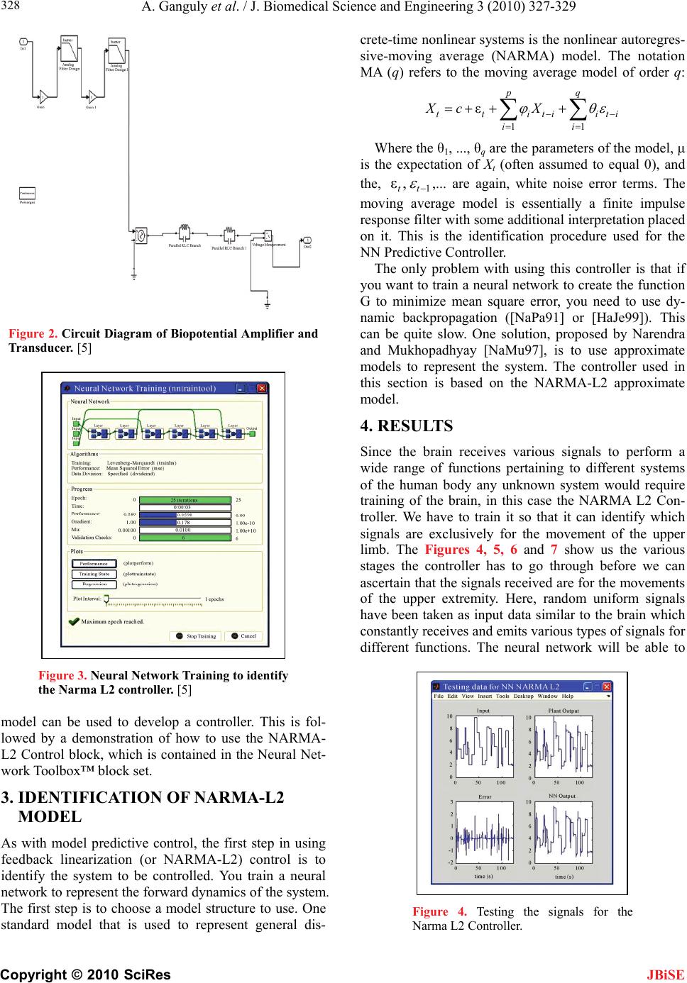
The Figure 1 above shows the arrangement of the circuit
components of the Model of Bionic Arm. [2,3]The uni-
form random signal goes to the brain that is the Narma
L2 Controller which goes to the subsystem of bionic arm
which consists of the biopotential amplifier and the
transducer, Figure 2 shown below. The graphical result
is viewed in the scope.
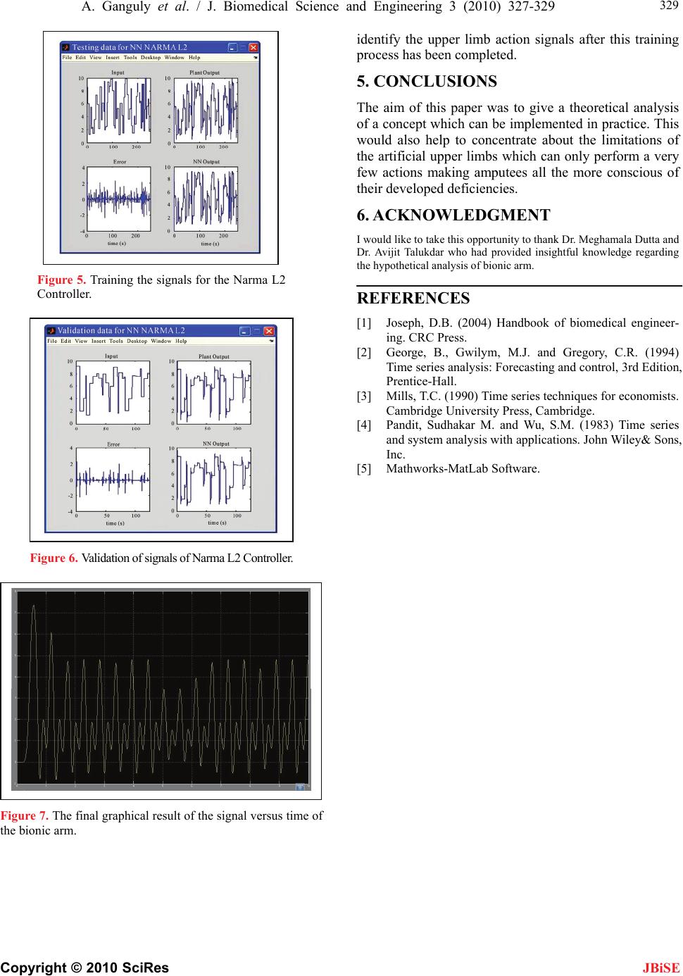
2.2. Narma L2 Controller
[4]The neurocontroller described in this section is re-
ferred to by two different names: feedback linearization
control and NARMA-L2 control. It is referred to as
feedback linearization when the plant model has a par-
ticular form (companion form). It is referred to as
NARMA-L2 control when the plant model can be ap-
proximated by the same form. The central idea of this
type of control is to transform nonlinear system dynam-
ics into linear dynamics by canceling the nonlinearities.
Figure 3 represents the training to identify the Narma
L2 controller. This section begins by presenting the
companion form system model and demonstrating how
you can use a neural network to identify this model.
Then it describes how the identified neural network
Figure 1. Block diagram of bionic arm. [5]

A. Ganguly et al. / J. Biomedical Science and Engineering 3 (2010) 327-329
328
JBiSE
Figure 2. Circuit Diagram of Biopotential Amplifier and
Transducer. [5]
Figure 3. Neural Network Training to identify
the Narma L2 controller. [5]
model can be used to develop a controller. This is fol-
lowed by a demonstration of how to use the NARMA-
L2 Control block, which is contained in the Neural Net-
work Toolbox™ block set.
3. IDENTIFICATION OF NARMA-L2
MODEL
As with model predictive control, the first step in using
feedback linearization (or NARMA-L2) control is to
identify the system to be controlled. You train a neural
network to represent the forward dynamics of the system.
The first step is to choose a model structure to use. One
standard model that is used to represent general dis-
crete-time nonlinear systems is the nonlinear autoregres-
sive-moving average (NARMA) model. The notation
MA (q) refers to the moving average model of order q:
11
ε
pq
ttitii
ii
XcX ti




 

Where the θ1, ..., θq are the parameters of the model, μ
is the expectation of Xt (often assumed to equal 0), and
the, 1 ε,
tt


,... are again, white noise error terms. The
moving average model is essentially a finite impulse
response filter with some additional interpretation placed
on it. This is the identification procedure used for the
NN Predictive Controller.
The only problem with using this controller is that if
you want to train a neural network to create the function
G to minimize mean square error, you need to use dy-
namic backpropagation ([NaPa91] or [HaJe99]). This
can be quite slow. One solution, proposed by Narendra
and Mukhopadhyay [NaMu97], is to use approximate
models to represent the system. The controller used in
this section is based on the NARMA-L2 approximate
model.
4. RESULTS
Since the brain receives various signals to perform a
wide range of functions pertaining to different systems
of the human body any unknown system would require
training of the brain, in this case the NARMA L2 Con-
troller. We have to train it so that it can identify which
signals are exclusively for the movement of the upper
limb. The Figures 4, 5, 6 and 7 show us the various
stages the controller has to go through before we can
ascertain that the signals received are for the movements
of the upper extremity. Here, random uniform signals
have been taken as input data similar to the brain which
constantly receives and emits various types of signals for
different functions. The neural network will be able to
Figure 4. Testing the signals for the
Narma L2 Controller.

A. Ganguly et al. / J. Biomedical Science and Engineering 3 (2010) 327-329
329
JBiSE
[5] Mathworks-MatLab Software.
identify the upper limb action signals after this training
process has been completed.
5. CONCLUSIONS
The aim of this paper was to give a theoretical analysis
of a concept which can be implemented in practice. This
would also help to concentrate about the limitations of
the artificial upper limbs which can only perform a very
few actions making amputees all the more conscious of
their developed deficiencies.
6. ACKNOWLEDGMENT
I would like to take this opportunity to thank Dr. Meghamala Dutta and
Dr. Avijit Talukdar who had provided insightful knowledge regarding
the hypothetical analysis of bionic arm.
Figure 5. Training the signals for the Narma L2
Controller. REFERENCES
[1] Joseph, D.B. (2004) Handbook of biomedical engineer-
ing. CRC Press.
[2] George, B., Gwilym, M.J. and Gregory, C.R. (1994)
Time series analysis: Forecasting and control, 3rd Edition,
Prentice-Hall.
[3] Mills, T.C. (1990) Time series techniques for economists.
Cambridge University Press, Cambridge.
[4] Pandit, Sudhakar M. and Wu, S.M. (1983) Time series
and system analysis with applications. John Wiley& Sons,
Inc.
Figure 6. V
alidation of signals of Narma L2 Controller.
Figure 7. The final graphical result of the signal versus time of
the bionic arm.