 J. Biomedical Science and Engineering, 2010, 3, 308-316 doi:10.4236/jbise.2010.33042 Published Online March 2010 (http://www.SciRP.org/journal/jbise/ JBiSE ). Published Online March 2010 in SciRes. http://www.scirp.org/journal/jbise An index for evaluating distance of a healthy heart from Sino-Atrial blocking arrhythmia Hossein Gholizade-Narm1, Morteza Khademi2, Asad Azemi3, Masoud Karimi-Ghartemani4 1Electronic & Robotic Engineering, Shahrood University Technology, Shahrood, Iran; 2Ferdowsi University of Mashhad, Mashhad, Iran; 3College of Engineering, Penn State University, Philadelphia, USA; 4Sharif University of Technology, Tehran, Iran. Email: Gholizade@shahroodut.ac.ir Received 29 November 2009; revised 15 December 2009; accepted 28 December 2009. ABSTRACT In this paper, an index for evaluating Distance of a healthy heart from Sino-Atrial Blocking Arrhythmia (SABA) is presented. After definition of the main pacemakers' model of heart, Sino-Atrial (SA) and Atrio-Ventricular nodes (AV), the boundary of syn- chronization, which demonstrates the boundary of blocking arrhythmia, is obtained using perturbation method. In order to estimate of healthy heart char- acteristics, a parameter estimator is introduced. The distance from SABA is calculated using Lagrange method and Kohn-Tucker conditions. In addition, the maximum admissible decrease in the coupling inten- sity and the maximum admissible increase in the dis- crepancy between the natural frequencies of two pacemakers are determined in order to maintain the synchronization between the two pacemakers. Keywords: Healthy Heart; Blocking Arrhythmia; Perturbation method; Synchronization Boundary; Optimization; Bifurcation 1. INTRODUCTION The heart arrhythmias are the first cause of death ac- cording to World Health Organization (WHO) reports [1]. The lack of information about the health degree is one of the many factors for this. In other words, if peo- ple know their relative degree of health, the demise will be decreased. Fortunately, the medical science has the ability to measure the distance from illness in many is- sues. For instance, the fat and glucose of blood can be determined by some easy checks. The treatment could be initiated if it was near dangerous zone. Many works have also been done on cardiac arrhythmias' prediction to reduce the cardiac sudden death. Most of them have been done by physicians. The statistical methods are often used in those researches. In statistical methods, the QRS complex and QT interval and other segments of Electro Cardio Graph (ECG) are investigated and car- diac sudden death is predicted [2,3,4,5]. The nonlinear features such as fractal dimensions of Heart Rate Vari- ability (HRV) are used by other methods to determine the risk of sudden death [6]. Finally, the General Regres- sion Neural Network (GRNN), Learning Vector Quanti- zation (LVQ) and wavelet transform are used to predict the life-threatening Ventricular tachycardia (VT) and Ventricular Fibrillation (VF) [7]. All of the works are based on signal processing and their result is a number which demonstrates the prob- ability of being prone to arrhythmia or death. Unfortu- nately, signal processing based methods are not of enough accuracy to predict life-threatening cardiac ar- rhythmias (less than 70%) [6,7]. On the other hand, it cannot evaluate the relative degree of health if the heart is assumed healthy. In this research, our goal is to evaluate the distance from SABA by observing action potential signals of SA and AV nodes. The blocking arrhythmias arise when two pacemakers are not in synchrony. The main reasons for asynchrony are either decreasing coupling intensity or increasing the discrepancy of two pacemakers' natural frequencies or both. For evaluation of distance from SABA, four stages should be passed. At first, a proper model should be considered for pacemakers. Then, the synchronization boundary must be obtained based on the model parameters. At the next stage, the model of pa- rameters should be estimated from pacemakers' action potentials. Finally, by defining a cost function for dis- tance from SABA and using optimization methods, the minimum distance is calculated. Many models have been proposed for pacemakers and heart cells till now. Among the most well-known of them are Van der Pol [8,9,10,11], Fitzhugh-Nagumo [12,13,14], Hodgkin-Huxley [15], Beeler-Reuter [16] and Lou-Rudy [17] model. In this research, the Van der  H. Gholizade-Narm et al. / J. Biomedical Science and Engineering 3 (2010) 308-316 Copyright © 2010 SciRes 309 JBiSE Pol model is used as the model of SA and AV nodes for its simplicity and sufficiency for synchronization issues. Synchronization and its boundary have dedicated many works of engineers and physicists to itself from the past decades. Synchronization can be divided into complete synchronization, lag synchronization, func- tional synchronization, phase synchronization and fre- quency synchronization [18,19]. The output signal of the oscillators must be exactly equal for complete synchro- nization. In other words, two signals should be identical in amplitude and frequency. The lag synchronization is similar to complete synchronization except that the out- put of one oscillator should be coincided on the delayed signal of another one. The complete and lag synchroni- zation are accessible only for two identical oscillators. In functional synchronization, the output signal of one os- cillator is a function of another one. This type of syn- chronization is defined for those oscillators whose pa- rameters are related together. Any type of the aforemen- tioned synchronization types will not be occurred if two oscillators are non-identical. However, most of the cou- pled oscillators are non-identical in nature. In this case, the phase and frequency synchronization is defined in which, the coincidence of the output signals of two os- cillators is not necessary. In phase synchronization, the phase difference of signals should be fixed for all the time and for frequency synchronization, it is enough that the phase difference of two oscillators to be bounded. The heart pacemakers are in phase synchrony in normal mode. When they tend to asynchrony, they pass fre- quency synchronization at first and then become asyn- chrony. Therefore, the boundary of synchronization is determined by frequency synchronization, but since it is difficult to find the frequency synchronization boundary (it can only be obtained by simulation [20]) and on the other hand, its distance from phase synchronization boundary if very tiny [20,21], the phase synchronization has been taken as arrhythmia boundary in this research. Perturbation methods, specially averaging method and bi-variant expansion are more applied in synchronization boundary determination [20,21,22]. The dynamical equa- tions of two coupled oscillators are mapped to polar space using perturbation method. In polar space, the phase difference of two oscillators is a state variable. Therefore, the stability of new dynamical system is suf- ficient for phase synchronization because, in this case, the phase difference tends to a fixed point. Unfortunately, there is not any background about measuring distance from arrhythmia. Our goal in this research is to evaluate this distance using synchroniza- tion boundary and pacemakers' parameters. In addition, we will answer to two questions: 1) How much the cou- pling intensity can be decreased subject to synchroniza- tion? 2) How much the natural frequency difference of two pacemakers can be increased subject to synchroni- zation? The paper is organized as follow: After introduction in Section 1, the synchronization boundary is obtained us- ing perturbation method in Section 2. A state and pa- rameter estimator is introduced in Section 3 for two cou- pled pacemakers system. The distance from SABA is evaluated in Section 4 and the maximum permitted value of natural frequency difference and minimum permitted value of coupling intensity are calculated in Section 5. Simulation results are demonstrated in Section 6 and the conclusion is discussed in Section 7. 2. THE PACEMAKER MODEL AND SYNCHRONIZATION BOUNDARY The asynchrony between two vital pacemakers, SA and AV nodes, is the basic reason of blocking arrhythmias. In a healthy heart, the relationship between these two pacemakers is unidirectional coupling (from SA node to AV node) according to physicians' opinion; however, some physiologists suggest that the relationship is bidi- rectional but the effect of AV node on SA node is very smaller than vice versa [23]. According to the feedback of automatic nerves, the second idea is more acceptable. Here, we take the coupling as bidirectional, which is the general form. To change bidirectional case to unidirec- tional case, it is sufficient to equate the correspondence coefficient to the effect of AV node on SA node to zero. The model of two coupled pacemakers using Van der Pol Equations are, 22 111 1 ttttt t xx xyx (1) 22 222 1 ttttt yyyyx t y (2) were 1 and 2 are damping coefficients, 1 and 2 are natural frequencies, and 1 and 2 are cou- pling coefficients which demonstrate coupling intensity. Assume Eqs. 1 and 2 are the SA and AV nodes' model respectively. According to relation between two coupled pacemakers, we take 12 ,1 . For using per- turbation method, the system should be transformed to perturbation standard form. By scaling the time as 1 tt which results 1 1, t dx 1 1 dt dx x dt dt dt 1 2 1 t x the Eqs. 1 and 2 change as, 11111 11111 2 12 2 22 1 11 ttttt ttttt xxxxyx yyyyx 1 t y (3)  310 H. Gholizade-Narm et al. / J. Biomedical Science and Engineering 3 (2010) 308-316 Copyright © 2010 SciRes JBiSE where 22 22 12 1, 1 2 and 2 . Sup- pose 11 1 therefore 1 . On the other hand, k . Remark: the natural frequency of SA node is greater than AV node in the healthy heart. Since our goal is the measurement of the distance of healthy heart from SABA, therefore according to 3. 0 Consider variables x and y linear versus as 01 0 ,1 xxyyy . By bi-variant expanding of Eq. 3 versus time in the form of 11 ,tt 2 O and eliminating higher order terms ( and higher terms) we have, 2 0 0 20 xx (4) 2 2 2 00 1 10 21 21 x xxx (5) 2 0 0 20 yy (6) 2 2 2 00 1 10 22 00 20 21 yy yxy xy y (7) Considering x0 and y0 in periodic forms, 0 0 cos sin cos sin xA B yC D (8) By substituting x0 and y0 at the right hand of Eqs. 4 and 6 and equating secular terms (coefficients of sin and cos ) to zero we have, 22 11 22 11 1 24 1 24 dA AA B d dB BBAB d (9) 22 22 2 22 22 2 1 24 1 24 dC CCCD DB d dD DDCD AC d D C (10) Define A, B, C and D as follow, 11 11 22 22 cos ,sin cos ,sin AR BR CR DR (11) Therefore, x0 and y0 are, 01 1 02 2 ,cos ,cos xR yR (12) By substituting A, B, C and D in 9 and 10 and rear- ranging them, 2 111 1 11 2 2222 2112 2222 112 1 21 4 20 1 21 sin 4 2cos RR R R RRR R RR (13) where 121 1212 ,,, dRdR dd RR ddd 2 d . Assume 12 , the slow flow dynamical Equations are, 2 111 1 2 2222 21 1 22 2 1 21 4 1 21s 4 2co RR R RRRR R R in s (14) where 12 d d . The synchronization boundary is achieved by determining the Saddle-Node (S-N) and Hopf bifurcation condition curves of 14 [20]. The first step is to find the equilibrium points curve. Equate the left hand of 14 to 0, 2 11 11 1 10 4 RR R 2 (15) 2 222 21 2 22 2 21 1 1sin 4 1 14 sin RRR RR R 0 (16)  H. Gholizade-Narm et al. / J. Biomedical Science and Engineering 3 (2010) 308-316 Copyright © 2010 SciRes 311 JBiSE 1 22 2 22 21 cos 0 cos R R R R (17) By summing the square of 16 and 17 and substituting R1=2 we have, 2 2 2 2222 22 1 1 4 RRR 2 4 p (18) Replace and rearrange 18 according to power of p, 2 2 R 2 23 2222 22 222 11 4 16 2 pp p 0 (19) Eq. 19 shows the curve of equilibrium points vs. the system's parameters. Using Descartes’ rule of signs we see that (19) has either one or three positive roots for p. At bifurcation, there will be a double root which corre- sponds to requiring the derivative of (19) to vanish: 2 22 22 22 22 30 16 pp (20) Eliminating p from (19) and (20) gives the condition for S-N bifurcation as, 65224 23 222222 44 222 22 22 4523624 22222222 4246083280 604 12 82440 40 3 (21) Eq. 21 plots as two curves intersecting at cusp points in the plane. At the cusp point, a further degen- eracy occurs and there is a triple root in Eq. 19. Deriva- tion from 20 gives, 2, 8 3 p (22) By substituting p from (22) to (19) and (20) gives cusp points. 221 222 0.544 ,0.033, 0.544 ,1.122 2 2 (23) Next we look for Hopf bifurcations in the slow flow system 14. Let be an equilibrium point. The behavior of the system linearized in the neighbor- hood of this point is determined by the eigenvalues of the Jacobian matrix. 10 20 0 ,,RR 2 10 1 2 20 2021020 210 210 2 00 2 20 20 20 34 00 4 34 1sin cos 24 cos cossin R R JR RR RR R 0 (24) Substituting 00 sin,cos, R 10 from (15–17) in 24 and after simplification, 1 22 222202220 222 220 20 200 11 13 11 22 44 1 1 24 RR RR R R (25) For Hopf bifurcation, it is necessary that matrix J con- tains 2 pure imaginary and 1 real eigenvalue. 22 1220222332332 0 10 2 IJ RJJJJ (26) It can be seen from 26 that the coefficient of must be 0 for Hopf bifurcation. 2 220220 10 2RpR 2 2 (27) Substituting p from 27 in Eq. 19 gives the Hopf bi- furcation condition curve. 22 222 1 20 4 2 (28) Eqs. 21 and 28 identify the phase synchronization boundary. A typical sample for synchronization bound- ary is brought in Ex. 1. Synchronization boundary Equations show that the boundary depends on coupling coefficients, damping coefficients and discrepancy of two pacemakers’ natural frequency. Therefore, they should be estimated in prac- tice for distance evaluation from SABA. 3. THE STATE-PARAMETER ESTIMATOR Measurement of all states and parameters of the cardiac pacemakers is impossible in practice but the measure- ment of only their action potentials is practical using two implantable leads. In this section, a state-parameter es- timator (adaptive observer) is introduced which is able to  312 H. Gholizade-Narm et al. / J. Biomedical Science and Engineering 3 (2010) 308-316 Copyright © 2010 SciRes The adaptive rules are, estimate necessary parameters from pacemakers' action potentials for distance evaluation. This estimator uses the high-gain method. The high-gain method is very effective in state estimation [24]. When the parameters are unknown in addition to states, the estimator is modi- fied which is called adaptive observer. An adaptive ob- server is introduced in [25] which can estimate parame- ters and states simultaneously. We use an adaptive ob- server which is introduced in [25] in this research. The system form is as follow, JBiSE 1 1 2 1 1 2 1 2 , 0 , 0 , , 0 0 tut A xt xt tut A xt ut xt ut C yt xt C (29) 1 ˆˆ , ˆˆ ,, ˆ ˆ ˆˆ ,. ˆ ˆ ˆˆ ,. ˆ TT TT tAKCt xtut tAxtxt utxt utt KttCytCxt tI tCytCxt x xx ifxXXotherwise x if otherwise , (31) are the upper bound, 0, 0x 1 2 0 0 K K where where , , and n x 2 y q ,, ii i A are the state vector, output vector and the unknown parameters vector re- spectively. The matricesC , i = 1, 2 are, and K1,2 are selected such that the ii ,1 , 2 1 1 01 0 , 1 00 00 , 00 ,, 100 , ii i i i inin q ini i A xu ux Cnn i KC matrix be stable. 1 12 1,2 1 2 1,,,,0 , 0 0 i n idiag and 1 2 0 0 n n I I u (30) For using the introduced adaptive observer, the system 1 and 2 must be mapped to state space rep- resentation. ,, tAxtxt utxt ut yt Cxt (32) where,  H. Gholizade-Narm et al. / J. Biomedical Science and Engineering 3 (2010) 308-316 Copyright © 2010 SciRes 313 00 JBiSE 1234 22 11 1222 2 12113 2 34313 010 0 1000 0000 ,, 0010 0001 0000 ,, 0 000 000 10 , 000 000 0001 T T CAxtxtxtxt xt xu xtxt xt xtxt xu txtxtxtxt (33) The performance of introduced estimator is demon- strated in Ex. 2. 4. DISTANCE EVALUATION FROM SABA In this section, our goal is to evaluate the distance from SABA using synchronization boundary and pacemakers' parameters. As it was mentioned in Section 2, the boundary is determined by S-N and Hopf bifurcation conditions. If 2 1.122 0 , the boundary is de- termined by S-N bifurcation condition curve. Otherwise, the synchronization boundary is identified by Hopf bi- furcation condition curve. For distance evaluation, at first, the pacemakers' parameters should be mapped from 12 ,, , space to ,, space. 22 212 1 1,, 2 (34) The second step is to find a point on synchronization boundary in which has the minimum distance from . Assume the point ,, 22 ,, is the desired point. By inverse transformation of this point using (35), the minimum distance from SABA can be obtained. 22 2min 122 1 ,1 (35) 22 2 22min 2222 Min. Dist. from Blocking Arrh. (36) The crucial point is how to find the desired point. The Eq. 21 contains two curves that one of them pass through origin point (0, 0, 0) and forms the first part of synchroniza- tion boundary. For simplicity, we approximate this curve by a line which passes from origin and cusp point. (37) 20.48485 Therefore, the synchronization boundary is defined by Eqs. 28 and 37. Suppose 22 ,, PP P is the pacemakers' parameters which is transformed to ,, space. Define the distance of a point on boundary ,,Q from P as, 22 2 22 22 PP Dis 2 P (38) By minimizing 38 subject to 37 and again subject to 28 individually and taking into account their minimum value, the desired point is achieved. Therefore, two minimization problems should be solved. 22 ,, 2 122 2 2 . .,,0.484850 1.122 0 Minimize Dis ST f (39) Using Lagrange coefficient and Kohn-Tucker method for considering inequality constraints we have, 2 112212 , ,1.122LDis f 2 (40) 22 1 ,, 1 1 22 0 0 0 1.122 0 L L (41) 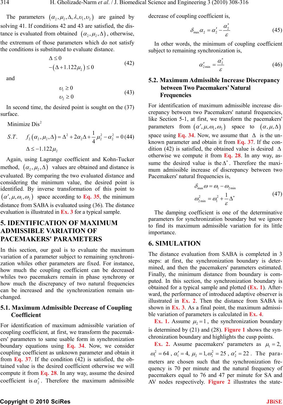 314 H. Gholizade-Narm et al. / J. Biomedical Science and Engineering 3 (2010) 308-316 Copyright © 2010 SciRes JBiSE The parameters 22 12 ,,,,, 22 are gained by solving 41. If conditions 42 and 43 are satisfied, the dis- tance is evaluated from obtained , otherwise, the extremum of those parameters which do not satisfy the conditions is substituted to evaluate distance. ,, 2 0 1.122 0 (42) and 1 2 0 0 (43) In second time, the desired point is sought on the (37) surface. 2 22 22222 2 2 Minimize Dis 1 .., ,20 4 1.122 ST f 2 (44) Again, using Lagrange coefficient and Kohn-Tucker method, values are obtained and distance is evaluated. By comparing the two evaluated distance and considering the minimum value, the desired point is identified. By inverse transformation of this point to 22 ,, 12 , ,, space according to Eq. 35, the minimum distance from SABA is evaluated using (36). The distance evaluation is illustrated in Ex. 3 for a typical sample. 5. IDENTIFICATION OF MAXIMUM ADMISSIBLE VARIATION OF PACEMAKERS' PARAMETERS In this section, our goal is to evaluate the maximum variation of a parameter subject to remaining synchroni- zation whiles other parameters are fixed. For instance, how much the coupling coefficient can be decreased whiles two pacemakers remain in phase synchrony or how much the discrepancy of two natural frequencies can be increased and the synchronization remain un- changed. 5.1. Maximum Admissible Decrease of Coupling Coefficient For identification of maximum admissible variation of coupling coefficient, at first, we transform the pacemak- ers' parameters to same usable form in synchronization boundary equations using Eq. 34. Now, we consider coupling coefficient as unknown parameter and obtain it from Eq. 37. If the condition (42) is satisfied, the ob- tained value is the desired coefficient otherwise we will compute it from Eq. 28. In any way, assume the desired coefficient is2 . Therefore the maximum admissible decrease of coupling coefficient is, 2 max22 (45) In other words, the minimum of coupling coefficient subject to remaining synchronization is, 2 2min (46) 5.2. Maximum Admissible Increase Discrepancy between Two Pacemakers’ Natural Frequencies For identification of maximum admissible increase dis- crepancy between two Pacemakers' natural frequencies, like Section 5-1, at first, we transform the pacemakers' parameters from 12 ,, , space to ,, space using Eq. 34. Now, we assume that is the un- known parameter and obtain it from Eq. 37. If the con- dition (42) is satisfied, the obtained value is desired otherwise we compute it from Eq. 28. In any way, as- sume the desired value is the. Therefore the maxi- mum admissible increase of discrepancy between two Pacemakers' natural frequencies is, max12 min 22 2min 1 1 (47) The damping coefficient is one of the determinative parameters for synchronization boundary but we ignore to find its maximum admissible variation for its little importance. 6. SIMULATION The distance evaluation from SABA is completed in 3 steps: at first, the synchronization boundary is deter- mined, and then the pacemakers' parameters estimated. Finally, the minimum distance from boundary is com- puted. In this section, the synchronization boundary is obtained for a typical sample and plotted (Ex. 1). After- ward, the performance of introduced adaptive observer is illustrated in Ex. 2. Then the distance from SABA is shown in Ex. 3. As a final point, the maximum admissi- ble variation of parameters is calculated in Ex. 4. Ex. 1. Assume 21 , the synchronization boundary is determined by (21) and (28). Figure 1 shows the syn- chronization boundary and highlights the cusp points. Ex. 2. Assume pacemakers' parameters as 12, 22 11222 64,4,1,25,2 2 . The para- meters are chosen such that the synchronization fre- quency is 70 per minute and the natural frequency of pacemakers equal to 76 and 47 per minute for SA and AV nodes respectively. Figure 2 illustrates the state- 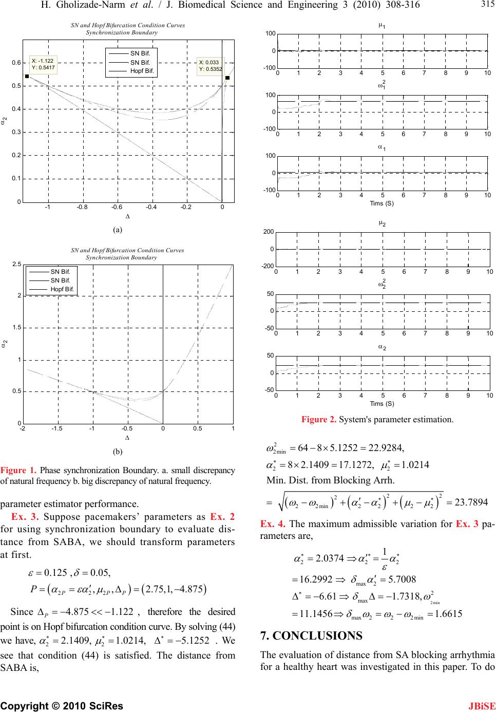 H. Gholizade-Narm et al. / J. Biomedical Science and Engineering 3 (2010) 308-316 Copyright © 2010 SciRes 315 JBiSE -1 -0.8 -0.6 -0.4 -0.20 0 0.1 0.2 0.3 0.4 0.5 0.6 X: 0.033 Y: 0.5352 SN and Hopf Bifurcation Condition Curves Synchronization Boundary 2 X: -1.122 Y: 0.5417 SN Bif. SN Bif. Hopf Bif. (a) -2 -1.5-1-0.5 00.5 1 0 0. 5 1 1. 5 2 2. 5 SN and Hopf Bifurcation Condition Curves Synchronization Boundary 2 SN Bif. SN Bif. Hopf Bif. (b) Figure 1. Phase synchronization Boundary. a. small discrepancy of natural frequency b. big discrepancy of natural frequency. parameter estimator performance. Ex. 3. Suppose pacemakers’ parameters as Ex. 2 for using synchronization boundary to evaluate dis- tance from SABA, we should transform parameters at first. 222 0.125 ,0.05, ,,2.75,1, 4.875 PPP P Since , therefore the desired point is on Hopf bifurcation condition curve. By solving (44) we have,. We see that condition (44) is satisfied. The distance from SABA is, 4.875 1.122 P 22 2.1409, 1.021 4, 5.1252 0 1 23 45 678 910 -100 0 100 1 0 1 23 45 678 910 -100 0 100 1 2 0 1 23 45 678 910 -100 0 100 1 Tims (S) 012345678910 -200 0 200 2 012345678910 -50 0 50 2 2 012345678910 -50 0 50 2 Tims (S) Figure 2. System's parameter estimation. 2 2min 22 22 2 22min22 22 648 5.125222.9284, 8 2.140917.1272,1.0214 Min. Dist. from Blocking Arrh. 23.7894 Ex. 4. The maximum admissible variation for Ex. 3 pa- rameters are, 2min 222 max2 2 max max222 min 1 2.0374 16.2992 5.7008 6.61 1.7318, 11.1456 1.6615 7. CONCLUSIONS The evaluation of distance from SA blocking arrhythmia for a healthy heart was investigated in this paper. To do  316 H. Gholizade-Narm et al. / J. Biomedical Science and Engineering 3 (2010) 308-316 Copyright © 2010 SciRes this, the synchronization boundary was obtained using perturbation method. The synchronization boundary de- fines the illness boundary approximately. To compute the distance from this boundary, an estimator was intro- duced which can estimate SA and AV nodes’ parameters from their action potential signals. Using optimization methods, the minimum distance from SABA was evalu- ated. This value can be considered as an alarm when it is very small. The coupling intensity and discrepancy of natural frequency of two pacemakers play a crucial role in synchronization of two basic pacemakers. Hence, a method was proposed to evaluate the maximum admis- sible variation of these parameters. The maximum varia- tion value demonstrates the confidence margin. [10] Grudzinsky, K. and Zebrowski, J. (2004) Modeling car- diac pacemakers with relaxation oscillators. Physica A: Statistical Mechanics and its Applications, 153-162. [11] Sato, S., Doi, S. and Nomura, T. (1994) Bonhoffer-van der pol oscillator model of the Sino-Atrial node: A possi- ble mechanism of heart rate regulation. Method of In- formation in Medicin, 116-119. [12] Fitzhugh, R. (1961) Impulses and physiological in theo- retical models of nerve membranes. Biophysical Journal, 1, 445-466. [13] FitzHugh, R. (1969) Mathematical models of excitation and propagation in nerve. In: Schwan H.P. Ed., Biologi- cal Engineering, McGraw Hill, New York. [14] Nagumo, J., Arimoto, S. and Yoshizawa, S. (1962) An active pulse transmission line simulating nerve axon. Proceedings of the IRE, 50, 2061-2070. [15] Hodgkin, A. L., Huxley, A. F. and Katz, B. (1952) Meas- urement of current-voltage relations in the membrane of the giant axon of Loligo, The Journal of physiology, 116, 424. REFERENCES [1] World Helth Organization (WHO), Internet Available: www.who.int. [16] Beeler, G.W. and Reuter, H. (1977) Reconstruction of the action potential of ventricular myocardial fibres. The Journal of physiology, 268, 177-210. [2] El-Sherif, N., Denes, P., Katz, R., Capone, R., Brent , L., Carlson, M. and Reynolds, R. (1995) Definition of the best prediction criteria of the time domain sig- nal-averaged electrocardiogram for serious arrhythmic events in the post infraction period. Journal of American Collection Cardiology, 25(4), 908-914. [17] Lou, C.H. and Rudy, Y. (1994) A dynamic model of the cardiac ventricular action potential I. Circulation Re- search, 74, 1071-1096. [18] Pikovsky, A., Rosenblum, M. and Kurths, J. (2002) Syn- chronization: A universal concept nonlinear science, Cambridge University Press. [3] Tsagalou, E. P., Anastasiou-Nava, M. I., Karagounis, L. A., Alexopoulos, G. P., Batziou, C., Toumanidis, S., Pa- padaki, E. and Nanas, J. N. (2002) Dispersion of QT and QRS in patients with severe congestive heart failure: Re- lation to cardiac and sudden death mortality, Hellenic Jornal of Cardiology, 43, 209-215. [19] Santos, A. M., Lopes, S. R. and Viana, R. L. (2004) Rhythm synchronization and chaotic modulation of cou- plead van der pol oscillatiors in a model for the heartbeat. Physica A, 338, 335-355. [4] Thong, T., McNames, J., Aboy, M. and Goldstein, B. (2003) Paroxysmal atrial fibrillation prediction using isolated premature atrial events and paroxysmal atrial tachycardia. Proceedings of IEEE International Confer- ence on Biomedical Engineering, EMBC, 163-166. [20] Rand R. H. (2004) Lecture notes in nonlinear vibrations. 45 version, The Internet-First University Press, Ithaca. http://dspace.library.cornell.edu/handle/1813/79. [21] Rompala, K., Rand, R. and Howland, H. (2007) Dynam- ics of three coupled van der Pol oscillators with applica- tion to circadian rhythms. Communications in Nonlinear Science and Numerical Simulation, 12, 794-803. [5] Thong, T., McNames, J., Aboy, M. and Goldstein, B. (2004) Prediction of paroxysmal atrial fibrillation by analysis of atrial premature complexes. IEEE Transac- tions On Biomedical Engineering, 51(4), 561-569. [22] Nayfeh, A. H. (1973) Perturbation Methods, John Wiley & Sons Ltd., Chichester. [6] Owis, I., Abou-Zied, H. and Youssef, M. (2002) Study of Features Based on Nonlinear Dynamical Modeling in ECG Arrhythmia Detection and Classification. IEEE Trans- actions On Biomedical Engineering, 49(7), 733-736. [23] Grudzinski, K., Zebrowski, J.J. and Baranowski, R. (2006) Model of the sino-atrial and atrio-ventricular nodes of the conduction system of the human heart. Bio- medical Technology, 51, 210-214. [7] Abbas, R., Aziz, W. and Arif, M. (2004) Prediction of ventricular Tachyarrhythmia in Electrocardiograph Sig- nal Using Neuro-wavelet Approach. National Conference on Emerging Technologies, 82-87. [24] Gauthier, J. P., Hammouri, H. and Othman, S. (1992) A simple observer for nonlinear systems – applications to bioreactors. IEEE Transactions on Automatic Control. 37(6), 875-880. [8] V an der Pol, B. and Van der mark, J. (1927) Frequency demultiplication. Nature, 120, 363-364. [25] Besancon, G ., Zhang, Q. and Hammouri, H., (2002) High-Gain observer based state and parameter estimation in nonlinear systems. International Federation of Auto- matic Control. [9] V an der Pol, B. and Van der mark, J. (1928) The Heart- beat considered as a relaxation oscillation and electrical model of heart. Phil. Mag. Supll., 6, 763-775. JBiSE
|