J. Software Engineering & Applications, 2010, 3: 230-239
doi:10.4236/jsea.2010.33028 Published Online March 2010 (http://www.SciRP.org/journal/jsea)
Applying Neural Network Architecture for Inverse
Kinematics Problem in Robotics
Bassam Daya, Shadi Khawandi, Mohamed Akoum
Institute of Technology, Lebanese University, Saida, Lebanon.
Received November 12th, 2009; revised December 15th, 2009; accepted December 22nd, 2009.
ABSTRACT
One of the most important problems in robot kinematics and control is, finding the solution of Inverse Kinematics. Inverse
kinematics computation has been one of the main problems in robotics research. As the Complexity of robot increases,
obtaining the inverse kinematics is difficult and computationally expensive. Traditional methods such as geometric,
iterative and algebraic are inadequate if the joint structure of the manipulator is more complex. As alternative
approaches, neural networks and optimal search methods have been widely used for inverse kinematics modeling and
control in robotics This paper proposes neural network architecture that consists of 6 sub-neural networks to solve the
inverse kinematics problem for robotics manipulators with 2 or higher degrees of freedom. The neural networks utilized
are multi-layered perceptron (MLP) with a back-propagation training algorithm. This approach will reduce the
complexity of the algorithm and calculation (matrix inversion) faced when using the Inverse Geometric Models
implementation (IGM) in robotics. The obtained results are presented and analyzed in order to prove the efficiency of the
proposed a p proach.
Keywords: Inverse Geometric Model, Neural Network, Multi-Layered Perceptron, Robotic System, Arm
1. Introduction
The task of calculating all of the joint angles that would
result in a specific position /orientation of an end-effector
of a robot arm is called the inverse kinematics problem. In
the recent years, the robot control problem has received
considerable attention due to its complexity. Inverse
kinematics modeling has been one of the main problems
in robotics research, there has been a lot of research on the
use of neural networks for control The most popular
method for controlling robotic arms [1–5].
In inverse kinematics learning, the co mplexity is in the
geometric and non linear equations (trigonometric equa-
tions) and in the matrix inversion, this in addition to some
other difficulties faced in inverse kinematics like having
multiple solutions. The traditional mathematical solutions
for inverse kinematics problem, such as geometric, itera-
tive and algebraic, may not lead always to physical solu-
tions. When the number of manipulator degrees of free-
dom increases, and structural flexibility is included, ana-
lytical modeling becomes almost impossible. A modular
neural network architecture was proposed by Jacobs et al.
and has been used by many researches [2,3,5,6].
However, the input-ou tput relation of their networks is
continuous and the learning method of them is not suffi-
cient for the non-linearity of the kinematics system of the
robot arm.
This paper proposes neural network architecture for
inverse kinematics learning. The proposed approach con-
sists of 6 sub-neural networks. The neural networks util-
ized are multi-layered perceptron (MLP) with a back-
propagation training algorithm. They are trained with
end-effector position and joint angles.
In the sections that follow, we explain the inverse
kinematics problem, and then we propose our neural
network approach; we present and analyze the results in
order to p rove that neural networks prov ide a simple and
effective way to both model the manipulator inverse
kinematics and circumvent the problems associated with
algorithmic solution methods.
The proposed approach is presented as a strategy that
could be reused and implemented to solve the inverse
kinematics problems faced in robotics with highest de-
grees of freedom. The ba sics of this strategy are explained
in details in the section s th at follow.

Applying Neural Network Architecture for Inverse Kinematics Problem in Robotics231
2. Inverse Kinematics Pro ble m
Inverse kinematics computation has been one of the main
problems in robotics research. This problem is generally
more complex for robotics manipulators that are redun-
dant or wit h hi gh deg rees of freedom . Robot ki nemati cs is
the study of the motion (kinematics) of robots. They are
mainly of the following two types: forward kinematics
and inverse kinematics. Forward ki nematics is also k nown
as direct kinematics. In forward kinematics, the length of
each link and the a ngle of each joint are given and we have
to calculate the position of any point in the work volume
of the robot. In inverse kinematics, the length of each link
and position of the point in work vo lume is given and we
have to calculate the angle of each joi n. In thi s section, we
present the inverse kinematics problem.
2.1 Inverse Position Kinematics and IGM
The inverse position kinematics (IPK) solves the
following problem: “Given the desired position of the
robot’s hand; what must be the angles at the robot joints?”
In contrast to the forward problem, the solution of the
inverse problem is not always unique: The same end
effector’s pose can be reached in several configurations,
corresponding to distinct joint position vectors. The
conversion of the position and orientation of a robot
manipulator end-effector from Cartesian space to joint
space is called inverse kinematics problem. For any posi-
tion in the X-Y plane fo r a 2R robot, there is a possibility
of 2 solutions for any given point. This is due to the fact
that there are 2 configurations that might be possible to
reach the desired poi nt as Figure 1.
The math involved in solving the Inverse Kinematics
problem requires some background in linear algebra,
specifically in the anatomy and application of transfor-
mation matrices.
Therefore, an immediate attempt to solve the inverse
kinematics problem would be by inverting forward kine-
matics equations.
Let’s illustrate how to solve the inverse kinematics
problem for robot manipulators on a simple example.
Figure 2 shows a simple planar robot with two arms. The
underlying degrees of freedom of this robot are the two
angles dictating the rotation of the a rms. These are labeled
in Figure 2 as θ1 and θ2. The inverse kinematics question
in this case would be: What are the values for the degrees
of freedom so that the en d effector of t hi s r o bot (t he t i p o f
the last arm) lies at position (x, y) in the two-d imensional
Cartesian spac e ? One strai ght fo rwar d appr oa ch to s olvi ng
the problem is to try to write down the for ward ki nemat ics
equations that relate (x, y) to the two rotational degrees of
freedom, then try to solve these equations. This solution,
named IGM (Inverse Geometric Model) will give us an
answer to the inverse kinematics problem for this robot.
The calculation is presented in Figure 3.
As it can be seen in the example above, t he solutions t o
Figure 1. Two solutions depicted for the inverse kinematics
problem
Figure 2. Steer end-effector (x, y) target position
Figure 3. Finding solutions from the forward kinematics
equations
an inverse kine m ati cs proble m are not nece ssari ly unique.
In fact, as the number of degrees of freedom increases, so
does the m axim um number o f solutions , as depict ed in t he
figure. It i s also p ossible f or a pr oblem to have n o soluti on
if the point on the robot cannot be brought to the target
point in space at all.
While the above example offers equations that are easy
to solve, general inverse kinematics problems require
solving systems of nonlinear equations for which there are
no general al gorit hms . Som e inverse ki nema tics probl ems

Applying Neural Network Architecture for Inverse Kinematics Problem in Robotics 232
cannot be solved analytically. In robotics, it is sometimes
possible to design systems to have solvable inverse
kinematics, but in the general case, we must rely on ap-
proximation methods in order to keep the problem trac-
table, or, in some cases, even solvable.
It is known that there is a finite number of solutions to
the inverse kinematics problem. There are, however, 3
types of solutions: complete analytical solution, numerical
solutions and semi-analytical solution. In the first type, all
of the joint variables are solved analytically according to
given configuration data. In the second solution type, all
of the joint variables are ob tained iterative computatio nal
procedures. There are four disadvantages in these: 1)
incorrect initial estimations, 2) before executing the in-
verse kinematics algorithms, convergence to the correct
solution cannot be guaranteed, 3) multiple solutions are
not known, 4)there is no solution, if the Jacobian matrix is
singular. In the third typ e, some of the joint variables are
determined analytically and some computed numerically.
Disadvantage of numeric approaches to inverse kinemat-
ics problem is also heavy computational calculation and
big computational time.
3. Neural Network Approach
The true power and advantage of neural networks lies in
their ability to represent both linear and non-linear rela-
tionships and in their ability to learn these relationships
directly from the data being modeled. Traditional linear
models are simply inadequa te when it comes to mod eling
data that contains non-linear characteristics. The most
common neural network model is the multilayer percep-
tron (MLP). This type of neural network is known as a
supervised net wo rk because it re qui re s a desired o utp ut in
order to learn . The goal o f this ty pe of netw ork is to c reate
a model that correctly maps the inpu t to the output using
historical data so that the model can then be used to pro-
duce the output when the desired output is unknown. A
graphical representation of an MLP is shown in Figure 4.
The MLP and many other neural networks learn using
an algorithm called back propagation. With back
pr opa gation, the input data is repeatedly presented to the
neural network. With each presentation the output of the
Figure 4. A two hidden layer multiplayer perceptron (MLP)
neural network is compared to the desired output and an
error is computed. This error is then fed back (back
propagated) to the neural network and used to adjust the
weights such that the error decreases with each iteration
and the neural model gets closer and closer to producing
the desired output. This process is known as “training”.
As mentioned previously, for any position in the X-Y
plane for a 2R robot, there is a possibility of 2 solutions,
so our approach started by implementing one sub-net-
works for each solution. For each network, we will try to
obtain from the DGM model a series of q1(or θ1) and
q2(or θ2) for a given position of the end-effector. The data
training for the 2 sub-networks will be constructed as
following:
 Neural Network NN 1 : (x, y)  ( q1, q2);
o q1 between 0 and 2π, and q2 between 0 and π.
 Neural Network NN 2 : (x, y)  ( q1, q2);
o q1 between 0 and 2π, but q2 between -π and 0.
As we are going to use DGM for generating our input
parameters for the MLP (q1 and q2), for singular con-
figurations, for the same point X and Y, there are two
solutions for it within the same aspect. For example, as
shown in Figure 5, for 2 close positions of (x, y) we have
big difference in q1 values (first value of q1 is close to 0
and the other q1 is close to 2π). Thus, this will create a
problem during training for our data.
So the above implementation (2 neural networks) leads
to a big difficulty in the learning process. In order to
solve this problem, we will use 4 Neural Networks
(MLP); one for each quadrant.
By implementing 4 Neural Networks (MLP), we pre-
vent two main problems: 1) no more problem to con-
struct the training data for each aspect, and 2) no more
problem in the learning phase (one output for one input).
For the error there will be two other Neural Networks:
 One for the Cartesian space (MLP5), used to clas-
sify whether the given position is within or not in the
accessible region. The error will be representing whether
the given solution is within the limitation of the robots.
 One for the joint space (MLP6) to respect the joint
limit s of ou r robot.
The approach will use the schematic of the neural
network architecture given in Figure 6. The DGM model
is used to handle the problem of identifying which MLP
from the four MLPs is giving the right answer.
Figure 5. Two close positions for (x, y) but too different
values for q1 (0 and 2π) and this is for the same Neural
Network NN1 (q2 > 0)

Automated Identification of Basic Control Charts Patterns Using Neural Networks 233
Figure 6. Multi-layer perceptron architecture using 4 MLPs (1 to 4) for the 4 quadrants, MLP5 for the Cartesi an space and
MLP6 for the joint space. Qi represent the output (q1, q2) for MLPi (i = 1 to 4) and ERi represent the error output ( if ERi = 0
hen Qi accepted; if ERi = 1 then Qi rejected). t
4. Training, Experiments and Results
In this section, we present the configuration and prepar-
ing of the neural network, and the experiments, with their
results, executed in this approach.
We will use 6 MLPs to solve this problem. There will
be 1 MLP for each quadran t of the joint space , as shown in
Figure 7, mainly for q1 positive and q2 positive, q1 nega-
tive and q2 positive, q 1 positiv e an d q2 negativ e and lastly
q1 negative and q2 negative. For the error there will be 2
other neural networks: one to classify whether the given
position is within accessible region and one for the joint
space.
4.1 Creating MLP Network for IGM of 2R
Planar Robot
As mentioned above, for any position in the X-Y plane
for a 2R robot, there is a possibility of 2 solutions for any
given point. The appro ach will try to obtain a series of q 1
and q2 for a given position of the end-effecto r in the X-Y
plane. This is due to the fact that there are 2 configura-
tions that might be possible to reach the desired point.
For this MLP problem, we will be using 12 neurons for
the first layer and 8 neurons for the second layer and 2
neurons for t he output. H owever, the di fference is t hat we
will be using 6 MLPs to solve this problem. There will be
1 MLP for each quadrant of the joint space, as shown in
Figure 7, mainly for (q1 > 0 and q2 > 0), (q1 > 0 and q2 <
0), (q1 < 0 and q2 > 0) and lastly (q1 < 0 and q2 < 0).
This is done due to the fact that we are going to use
DGM for generating our input parameters for the MLP(q1
and q2). For singular configurations, for the same point
Figure 7. X-Y plane in 4 quadrants
X and Y, there are two solutions for it within the same
aspect. For example, for q1 = π and q2= –π, they will have
the same X and Y for any value of q2. Thus, this will create
a problem during training for our data. Thus, to solve this
problem, we will be using one MLP for each quadrant of
data. For the error there is perceptron used to classify
whether the given X and Y is within accessible and non
accessible region. The error will be representing whether
the solution given is within the limitation of the robots.
For example, if we give a point inside the non-accessible
region o f the working spac e, the error will be 1 and –1 for
inside the accessible region.
For each quadrant, we created 10 variables for our
target between q1 = 0 to π and equivalently for q2. Then,
we will use the Direct Geometry Model (DGM) function
to generate the data training for our MLPs. The tansig
function, used in our MLPs, will have its input from +3 to
–3 and its output between +1 and –1. The input and
outp ut for the MLP is then scaled according to the tansig
function.
To achieve this, we m ultiply the input x by 2.5 such t hat,
we will obtain –3 < x·2.5 < 3 (the same for the 4 MLPs).
The other scaling is given in Table 1.

Applying Neural Network Architecture for Inverse Kinematics Problem in Robotics 234
Table 1. Scaling of the input y and the outputs q1 and q2 for
each MLP according to the tansig function
No.
MLP q1 q
2 Y
MLP1 –1 < (q1·2⁄π) – 1
< 1 –1 < (q2·2⁄π) – 1 < 1 –3 < (y·5) – 2 < 3
MLP2 –1 < (q1·2⁄π ) + 1
< 1 –1 < (q2·2⁄π– 1 < 1 –3< (y·5) + 2 < 3
MLP3 –1 < (q1·2⁄π) – 1
< 1 –1 < (q2·2⁄π) + 1 < 1 –3 < (y·5) – 2 < 3
MLP4 –1 < (q1·2⁄π) + 1
< 1 –1 < (q2·2⁄π) – 1 < 1 –3< (y·5) + 2 < 3
4.1.1 The First MLP for the First Quadrant
For the first quadrant, we created 10 variables for our
target between q1 = 0 to π and equivalently for q2. Then,
we will use our DGM2R function to generate the input for
our MLP. The input and output for the MLP is then scaled
according to the tansig function. The tansig function will
have its input from +3 to –3 and its output between +1 and
-1. To achieve this, will be dividing our output and mul-
tiplying our inputs with factors. The resulting input and
output of for the MLP is shown in Figure 8.
(a)
(b)
Figure 8. (a) Input for first quadrant MLP; (b) target output
for first quadrant MLP
It is shown as well in Figure 8 that the initial result
from our MLP prior to training. For our MLP, we will be
using “trainlm” function since it is faster and more accu-
rate in producing the result.
The MLP managed to produce accurate data with error
of 1.74 × 10-5 within 25 epochs. The result is then
plotted back to our target. Figure 9 shows the result for
the MLP restoring the data prior to scaling. From Figure 9,
we know that our MLP has managed to produce quite an
accurate result since the result of the MLP is pretty close
to our target values.
For this MLP, we have used learning rate equal to 0.2.
The performance of the MLP is shown in Figure 10.
4.1.2 The Second MLP for the Second Quadrant
In the second MLP for the second quadrant of the joint
limit, we will do the same algorithm for training the MLP.
We will input our data in the range of q1 from 0 to –2.8
and q2 from 0 t o π. We will then input our data to “tansig”
transfer function. The inputs and outputs as well the initial
output of ou r M LP are presented in Figure 11. Using t he
Figure 9. Result of the first quadrant MLP plotted onto the
target data
Figure 10. Performance result for this first MLP

Applying Neural Network Architecture for Inverse Kinematics Problem in Robotics235
“trainlm” function, we managed to obtained accuracy of
1.38×10-5 within 41 epochs.
The result of the MLP is presented in Figure 12. The
result of the MLP presented is prior to rescaling back to
the original data. For the third MLP we will be performing
the similar operation by scaling the input and the output
before inputting it to the MLP to be learnt.
4.1.3 The Third MLP for the Third Quadrant
For the third MLP, we are trying to generate result for q1
in the range of 0 and π and q2 in the range of 0 to –2.8.
We are using –2.8 because of the requirement of the joint
limit present in the system. The initial input and output of
the system is presented in the following Figure 13.
After training our MLP for 15 epochs, we managed to
get an error in performance of 4.64 × 10-5 . The plot of
the result and the plot of the outputs are given in the fol-
lowing Figure 14.
4.1.4 The Fourth MLP for the Fourth Quadrant
For the last MLP to generate the result for IGM model, we
(a)
(b)
Figure 11. (a) Input data for the seco nd quadrant MLP; (b)
output of the second MLP plotted toge ther with the desired
result
are trying to generate result for q1 in the range of 0 and
–2.8 and q2 in the range of 0 to –2.8. For the same reason,
we are using –2.8 because of the requirement of the joint
limit present in the system. The initial input and output of
the system is presented in Figure 15. After training for 13
epochs, we managed to get an error of 5.24 × 10-5 and
the result of the MLP is plotted against the desired result.
We can observe that the resulting poi nts from the ML P are
close to the desired target. The result of the MLP and the
performance of the MLP are presented in Figure 16.
4.1.5 The Fifth MLP
The fifth MLP is designed to define the workspace of the
robot. The robot workspace is a circle with an internal
circle upon which the robot will not be able reach. Thus,
there is a limitation to the area upon which the robot is
able to access the area. When the given x and y is within
the internal circle or outside the working circle as depicted
in Figure 17, the error of the equation will be 1.
(a)
(b)
Figure 12. (a) Result of MLP plotted with the desired target;
(b) Performance of MLP with trainml function

Applying Neural Network Architecture for Inverse Kinematics Problem in Robotics 236
(a)
(b)
Figure 13. (a) Input for the 3rd MLP; (b) output of the 3rd
LP plotted with the desired result M
In order to do this, we will find the relationship be-
tween the length of the robots arms to the radius of its
working space. We know that the radius of the large cir
cle is given by the formula R=L1+L2. Thus, we know that
within the gray circle, . Expanding the
equation, we know that .
2
1
()RL L
21
12 2
2(RLL
2
2
0
2
2
)LL
Thus, we notice that if the desired point is within the
gray area, the value o f the equation above will be less
than 0, and otherwise if the value of R is smaller than L1
－L2 or R is greater than L1+L2.
We have created 20 numbers of data of X1 and X2 for
the input to the MLP.
Then, using t hese inputs, we c alculate our desired t arget
using the “error3” function using a notation that if error is
1 then the point is not inside working circle and if error is
0 then the robot is inside the work ing circle. The desired
target is presented in Figure 18. Our result shows that
(a)
(b)
Figure 14. (a) Output of the result plotted together with the
desired target of the 3rd MLP; (b) Performance of the 3rd
MLP
the MLP has managed to classify the classes within 17
epochs with zero error. Thus, this error problem has been
solved with only a single perceptron. The result of the
MLP is presented in Figure 18.
The performance of the perceprton is shown in Figure 19.
4.1.6 The Sixth MLP
The last step of the classification is to categorize the re-
sulting Q1 and Q2 into either [0 0] , [0 1] or [1 0]. This means
on the other hand, we need to classify the elements of
angles in the Q1 and Q2. If we draw the bound ary limit of
the angles, we would be able to find a rectangular area(as
shown in Figure 20). Certainly, we can apply the m e t hod
of perceptron with 3 layers for implementing classifier
arbitrary linearly limited areas (p olyhedron).
Thus, if our MLP is having 4 neurons on the first layer
and 1 neuron on the second layer and taking Q1 and Q2 as
the input para meters for the neur on and output of 1 i f Q1 or

Applying Neural Network Architecture for Inverse Kinematics Problem in Robotics237
(a)
(b)
Figure 15. (a) Input to the 4th MLP; (b) initial output of the
4th MLP plotted together with the desired result
Q2 is within the grey area and -1 if it outside the gray area,
we should be able to fully classify the problem.
The weights of our neurons are given as follows:
1
10
10
01
01
W








, and
1
3
2.8
3
2.8
b








Marking the desired area (grey area), we obtained
g
1 g 2 g 3 g 4
G1 - + - +
Thus,


211 11W , and .
2[3]b
From this weights and biases, our convention is :
 output = 1 if the value of Q is within the joint limit.
 output = -1 if t he value of Q i s outsi de the joint l imit.
(a)
(b)
Figure 16. (a) Performance of the 4th MLP; (b) Result of the
4th MLP plotted together with the desired target
With these values, we can create a MLP network and
we will be able to separate the two results perfectly. The
result is shown in Figure 21. Lastly, the final step is to
combine all the 6 MLP together in a program that we can
use to generate the desired Q1 and Q2 and error. We will
need to classify for the y of the input to our joint network.
Initially, when the input is having y > 0, there are two
solutions that are possible, which is q1 is positive and q2 is
positive or n egative. Thus, we have to choose quadrant 1
or 4 to obtain a correct result. Otherwise, when y < 0, the
two solutions that are possible are q1 is negative and q2 is
positive or negative. After we have done the classification,
then we can use our network to produce the desired result.
The program will check whether the given X and Y is
within the working circle. If it does not, then the error will
be equal to [1 1] and the value of Q1 and Q2 will be of a
null vector. On the other hand, if the point X, Y is within

Applying Neural Network Architecture for Inverse Kinematics Problem in Robotics 238
Figure 17. Working space of the robot
(a)
(b)
Figure 18. (a) Desired target result; (b) Result of the MLP
the circle, then it will input the X and Y according to the
given area as described above. Then, the resulting result
will be fed into the MLP 6 for determining whether the
result is within the joint limit or not. If it does, then error
will be equal to 0 and if it is not in the joint limit, then
error will be equal to 1.
Figure 19. Performance of the perceprton
Figure 20. Classification to categorize Q1 and Q2
Testing the MLP with values of
which corresponds to
[0.646 0.3196]X
[]
32
q


 , we obtained from
our MLP,


11.0936 1.6016Q
and


22.2538 1.5618Q
Our optimum result for the Q1 and Q2 from the IGM
model is


11.047 1.570Q
and


22.2232 1.5708Q
We know that the value from of MLP is pretty close to
the real values of the IGM2R model. The error is [0 0] and
[0 0] respectively.
Testing the MLP with values of
[ 0.31960.6464]X


which corresponds to 5 [
62
q]


 , we obtained from
our MLP,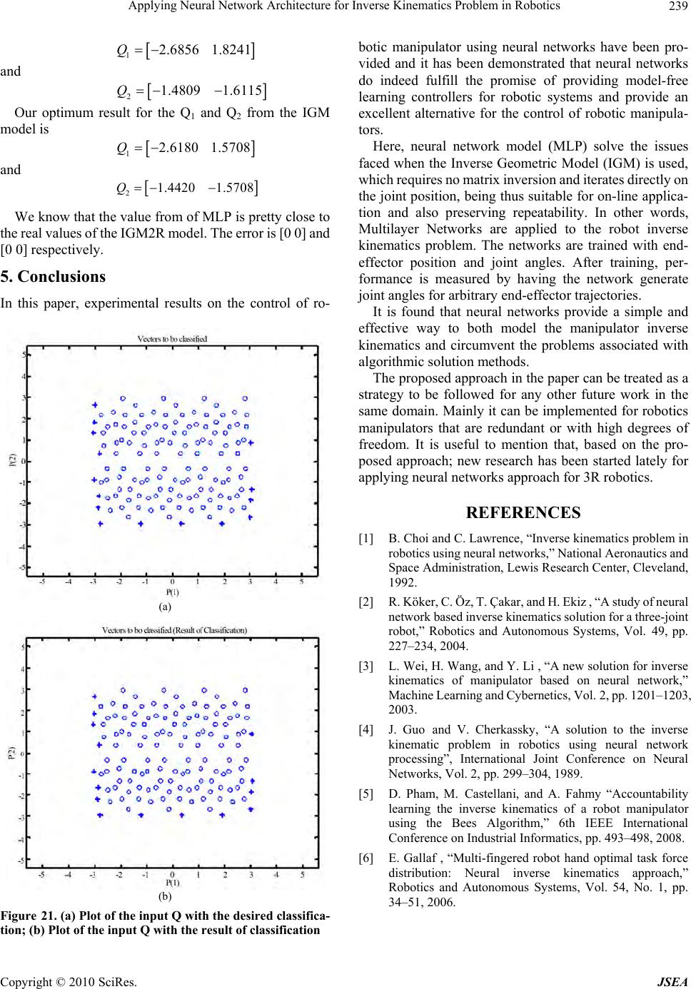

Applying Neural Network Architecture for Inverse Kinematics Problem in Robotics 239


12.6856 1.8241Q botic manipulator using neural networks have been pro-
vided and it has been demonstrated that neural networks
do indeed fulfill the promise of providing model-free
learning controllers for robotic systems and provide an
excellent alternative for the control of robotic manipula-
tors.
and


21.4809 1.6115Q
Our optimum result for the Q1 and Q2 from the IGM
model is


12.61801.5708Q Here, neural network model (MLP) solve the issues
faced when the Inverse Geometric Model (IGM) is used,
which requires no matrix inversion and iterates directly on
the joint position, being thus suitable for on-line app lica-
tion and also preserving repeatability. In other words,
Multilayer Networks are applied to the robot inverse
kinematics problem. The networks are trained with end-
effector position and joint angles. After training, per-
formance is measured by having the network generate
joint angles for arbitrary end-effector trajectories.
and


21.4420 1.5708Q
We know that the value from of MLP is pretty close to
the real values of the IGM2R model. The error is [0 0] and
[0 0] respectively.
5. Conclusions
In this paper, experimental results on the control of ro- It is found that neural networks provide a simple and
effective way to both model the manipulator inverse
kinematics and circumvent the problems associated with
algorithmic solution methods.
The proposed approach in the paper can be treated as a
strategy to be followed for any other future work in the
same domain. Mainly it can be implemented for robotics
manipulators that are redundant or with high degrees of
freedom. It is useful to mention that, based on the pro-
posed approach; new research has been started lately for
applying neural networks a p p roa ch for 3R roboti c s.
REFERENCES
[1] B. Choi and C. Lawrence, “Inverse kinematics problem in
robotics using neural networks,” National A eronautics and
Space Administration, Lewis Research Center, Cleveland,
1992.
[2] R. Köker, C. Öz, T. Çakar, and H. Ekiz , “A study of neur al
network based in verse kinem atics solution for a th ree-joint
robot,” Robotics and Autonomous Systems, Vol. 49, pp.
227–234, 2004.
(a)
[3] L. Wei, H. Wa ng, and Y. Li , “A new solution for inverse
kinematics of manipulator based on neural network,”
Machine Learnin g and Cybern etics, Vol. 2, pp. 1201–1203,
2003.
[4] J. Guo and V. Cherkassky, “A solution to the inverse
kinematic problem in robotics using neural network
processing”, International Joint Conference on Neural
Networks, Vol. 2, pp. 299–304, 1989.
[5] D. Pham, M. Castellani, and A. Fahmy “Accountability
learning the inverse kinematics of a robot manipulator
using the Bees Algorithm,” 6th IEEE International
Conference on Industrial Informatics, pp. 493–498, 2008.
[6] E. Gallaf , “Multi-fingered robot hand optimal task force
distribution: Neural inverse kinematics approach,”
Robotics and Autonomous Systems, Vol. 54, No. 1, pp.
34–51, 2006.
(b)
Figure 21. (a) Plot of the input Q with the desired classifica-
tion; (b) Plot of the input Q with the result of classification