Journal of Environmental Protection, 2010, 1, 1-9
doi:10.4236/jep.2010.11001 Published Online March 2010 (http://www.SciRP.org/journal/jep)
1
Modelling Livestock Activities and Environmental Sustainability:
The African Case
Eisa Abdalla Abdelgalil1, Suleiman Ibrahim Cohen2
1Economic Research Department, Dubai Chamber of Commerce and Industry, Dubai, UAE; 2Erasmus School of Economics, Eras-
mus University Rotterdam, Rotterdam, the Netherlands.
Received January 20th, 2010; revised February 28th, 2010; accepted March 1st, 2010.
ABSTRACT
This paper develops a dynamic model of grazing land degradation. The model illustrates the relationship between live-
stock levels and grazing land degradation over time. It identifies the mechanisms by which the factors internal to the
livestock local production system and those drawn from the larger economic context of livestock marketing influence
livestock-grazing land relationship. The paper shows that overstocking leads to degradation which leads to declining
relative prices of livestock as quality declines and mortality increases. As relative price of livestock falls, consumption
increases. The increased consumption and mortality ultimately leads to lower livestock population, which leads to de-
creased degradation. The model results show that medium term dynamics of grazing land degradation are quite differ-
ent from long term dynamics. It is shown that although grazing land sustainability situation is adverse in the medium
term, yet it is favourable in the long term. The livestock system is dynamic and can adjust when longer term system dy-
namics are allowed to play out. Part of the adjustment mechanism is built in the livestock system and the other part
comes from the economic system. The built-in adjustment mechanism works through the two-way relationship between
the stock and degradation. The external adjustment mechanism, originating from the economic system, works through
economic growth, relative prices and foreign trade. In the medium term, opportunistic management strategy and poli-
cies that facilitate access to grazing land and water are crucial for mitigating degradation. The results suggest that the
views of the mainstream range management paradigm and the new thinking of range ecology can be reconciled.
Keywords: Livestock, Grazing Land, Degradation, Models
1. Introduction
There are complex relationships between livestock graz-
ing and production on the one hand, and environment
conservation and degradation costs on the other hand. In
the context of the interaction between livestock and the
environment in developing countries, several studies
have underlined the tendency of overstocking of grazing
land resulting in land degradation, see [1–4].
The degradation of grazing land adversely affects the
natural growth rate of the livestock and its quality.
When grazing land is degraded, the stock fertility rate
falls and mortality rate rises, the weight of animals in
terms of kilograms is less and the quality of their prod-
uct is low, as compared to the situation where there is
no degradation. Also, when grazing land is degraded its
value falls. Furthermore, the decline in the livestock,
both in quantity and quality, and the fall of the value of
grazed land, lead to the decline of the capital wealth of
the livestock sector [5–8].
The empirical literature on the analysis of the trade-off
between livestock and environment and its economic
implications is very sporadic. There is no more than a
handful quantitative models that have addressed related
issues. Wilcox and Thomas [9] used for Australia a
model to examine the relationship between cost of pro-
duction and range conditions under long term steady-
state conditions. Braat and Opschoor [10] developed for
Botswana a simulation model that focused on the role of
rainfall and the stocking rate in determining the quality
of the range and herd development. Berrings and Stern
[11] using the cattle-rangeland system in the semi-arid
rangelands of Botswana, followed a dynamic economet-
ric approach for modelling the loss of resilience in an
ecological-economic system.
None of the above quoted research encroached on for-
malising and modelling the complex relationship be-
tween the various aspects of livestock activities and the
varied dimensions of environmental degradation. In this
paper, we develop a simple and at the same time a com-
prehensive model in nine equations, that examines the
medium and long terms dynamics of grazing and degra-

Modelling Livestock Activities and Environmental Sustainability: The African Case 2
dation in an African country, i.e. Sudan, where in relative
terms, livestock activities take significant proportions.
The importance of the model is that it synthesizes the
views of the mainstream range management paradigm
with the new range ecology thinking. The pursued model
integrates the ecological and economic dimensions of the
livestock system and the ecological system; these are
elements that are mostly missing in the literature. Em-
pirical data from Sudan are employed to operationalise
the model, and investigate the complex relationships and
their analytical and policy implications.
The paper proceeds as follows. Section 2 specifies the
model. Section 3 discusses its structure. Section 4 deals
with estimation and solution. Section 5 discusses the
model results for the medium term scenario over the pe-
riod 1990–2000, when livestock prices tended to fall in
relative terms. Section 6 discusses model results for a
long term scenario extending to 2030, where livestock
prices are assumed to remain stable in relative terms.
Section 7 examines sensitivity results, and Section 8 con-
cludes.
2. Model Specification
We formulate a determinate model of nine equations that
focuses on giving solutions to nine crucial variables that
link livestock activities and land degradation to each
other.
To start with, we denote the actual number of animal
stock that grazes on the available grazed land, by L. Next
to the actual grazing capacity, any grazing land can be
said to have an optimal carrying capacity for animals.
The optimal carrying capacity refers to the number of
animals that grazing land can support without being de-
graded. The word ‘optimal’ is used here in the agro-
nomical sense of the word. The optimal carrying capacity
of grazing land is determined by its size, N1, its annual
vegetation yield per unit of land, V, and the vegetation
requirement per animal unit, H. When the actual capacity
exceeds the optimal capacity, land degradation sets in.
This idea is formalised in Equation (1), where the nu-
merator gives the actual capacity, i.e. actual stock of ani-
mals, and the denominator gives the optimal capacity, i.e.
desirable stock of animals on grazing land.

1
1









Q
HNV
L
Q
t
(1)
In Equation (1), the ratio of the actual capacity to the
optimal one is used as an indicator of the prevailing con-
ditions on grazing land. This ratio is a degradation index
denoted by Q. The one-year lag of the variables is justi-
fied on the ground that it is the cumulative degradation
from last year that adversely affects the current year va-
riables.
When the actual capacity exceeds the optimal one, the
degradation index exceeds unity. Ideally, the actual ca-
pacity should approach the optimal one. The situation
when this is reached, i.e. Q = 1, will be seen that the
structure of the model will have to undergo changes that
will be treated in a later section. The situation where Q is
below unity, a process of grazing land and livestock re-
generation sets in, is not a focus of the paper.
According to Scoones [4] an effective management
strategy of Q can be achieved in four ways: 1) increasing
available fodder by enhancing its production or import-
ing feed from elsewhere; 2) moving livestock to where
fodder is available; 3) reducing animal feed intake during
drought through shifts in watering regimes; 4) destocking
animals through sales during drought. It can be seen from
Equation (1) that effective tracking is a good strategy that
can pre-empt or reduce grazing land degradation. This is
because increasing availability of fodder means increas-
ing V; moving animals to where fodder exists means ef-
fectively expanding N; reducing animal feed intake
means decreasing H; and destocking animals means re-
ducing L. All these four options lead to lower Q, or in
other words, less grazing land degradation.
Two of the four variables in the equation defining Q
are exogenously given; these are land N and vegetation
requirements H. The other two variables of V and L are
endogenous and their determination is displayed below in
additional equations.
The development of the vegetation yield of grazing
land, V, depends on three main factors: rainfall water,
Wrain, irrigation water2, Wirr, and degradation of graz-
ing land, Q. The influence of the abovementioned three
factors on vegetation yield is formalised in Equation (2).
V is positively related to the first two factors and in-
versely related to the third one. Given availability of rain
and irrigation water, the expected vegetation yield will
depend on the base year vegetation yield, v0, and on the
level of degradation of grazing land, as indicated by the
ratio of the degradation index in the base year Q0 to that
of the current year Q, and an elasticity parameter  .



 irrrain WW
QQ
v
V
0
0
(2)
The other variable to model is the size of the animal
stock on grazing land3 in the current year, L. This is de-
termined by last year’s stock, Lt-1, the natural growth rate,
g, and the slaughter from the stock, which is equivalent
to sale of livestock units of standard weight and quality
at a given price. X denotes the monetary value of live-
1The land unit used here is the feddan which is a measure of area and it is
equivalent to 4200 square metres or 0.42 acre.
2The term “irrigation water” is used here in its
b
road sense to refer to
underground water from dug wells as well as water from irrigation canals.
3Consideration is given here to four types of animals, namely, goats, sheep,
cattle and camels. This is because mainly these animals are consumed an
d
exported. Then, these animals are converted into livestock units (LSU)
using the following livestock unit conversion factors: sheep and goats a
t
0.12, cattle at 0.75 and camels at 1.00 [12].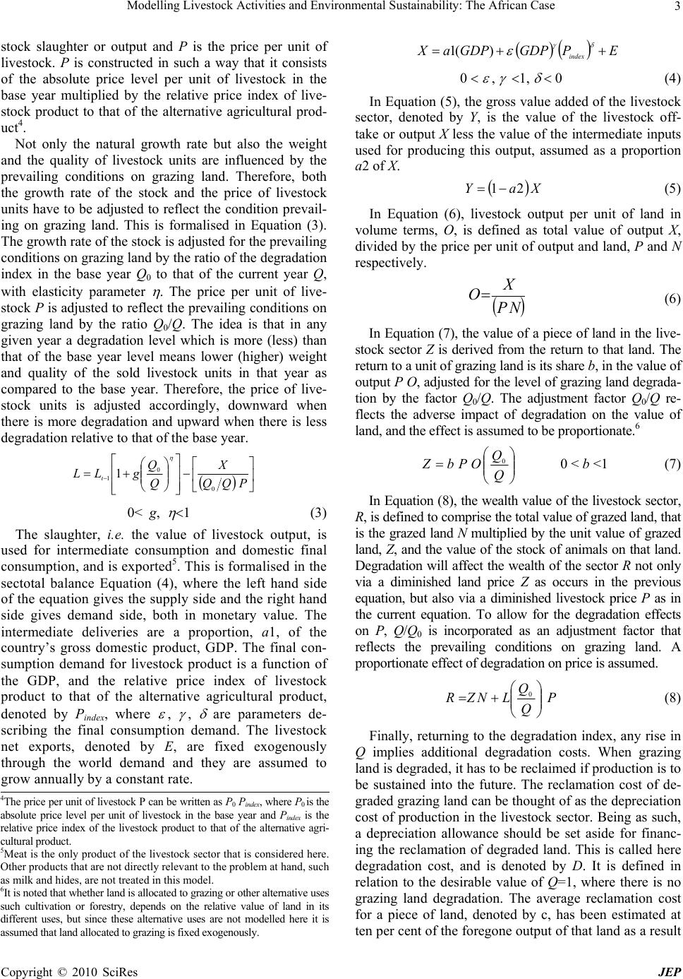

Modelling Livestock Activities and Environmental Sustainability: The African Case 3
stock slaughter or output and P is the price per unit of
livestock. P is constructed in such a way that it consists
of the absolute price level per unit of livestock in the
base year multiplied by the relative price index of live-
stock product to that of the alternative agricultural prod-
uct4.
Not only the natural growth rate but also the weight
and the quality of livestock units are influenced by the
prevailing conditions on grazing land. Therefore, both
the growth rate of the stock and the price of livestock
units have to be adjusted to reflect the condition prevail-
ing on grazing land. This is formalised in Equation (3).
The growth rate of the stock is adjusted for the prevailing
conditions on grazing land by the ratio of the degradation
index in the base year Q0 to that of the current year Q,
with elasticity parameter
 . The price per unit of live-
stock P is adjusted to reflect the prevailing conditions on
grazing land by the ratio Q0/Q. The idea is that in any
given year a degradation level which is more (less) than
that of the base year level means lower (higher) weight
and quality of the sold livestock units in that year as
compared to the base year. Therefore, the price of live-
stock units is adjusted accordingly, downward when
there is more degradation and upward when there is less
degradation relative to that of the base year.
























 PQQ
X
Q
Q
gLL t
0
0
11

0< g,
  (3)
The slaughter, i.e. the value of livestock output, is
used for intermediate consumption and domestic final
consumption, and is exported5. This is formalised in the
sectotal balance Equation (4), where the left hand side
of the equation gives the supply side and the right hand
side gives demand side, both in monetary value. The
intermediate deliveries are a proportion, a1, of the
country’s gross domestic product, GDP. The final con-
sumption demand for livestock product is a function of
the GDP, and the relative price index of livestock
product to that of the alternative agricultural product,
denoted by Pindex, where
 ,  ,  are parameters de-
scribing the final consumption demand. The livestock
net exports, denoted by E, are fixed exogenously
through the world demand and they are assumed to
grow annually by a constant rate.


EPGDPGDPaX index 

 )(1

      (4)
In Equation (5), the gross value added of the livestock
sector, denoted by Y, is the value of the livestock off-
take or output X less the value of the intermediate inputs
used for producing this output, assumed as a proportion
a2 of X.

 XaY 21


(5)
In Equation (6), livestock output per unit of land in
volume terms, O, is defined as total value of output X,
divided by the price per unit of output and land, P and N
respectively.
 NP
X
O (6)
In Equation (7), the value of a piece of land in the live-
stock sector Z is derived from the return to that land. The
return to a unit of grazing land is its share b, in the value of
output P O, adjusted for the level of grazing land degrada-
tion by the factor Q0/Q. The adjustment factor Q0/Q re-
flects the adverse impact of degradation on the value of
land, and the effect is assumed to be proportionate.6








Q
Q
OPbZ 0 0 < b <1 (7)
In Equation (8), the wealth value of the livestock sector,
R, is defined to comprise the total value of grazed land, that
is the grazed land N multiplied by the unit value of grazed
land, Z, and the value of the stock of animals on that land.
Degradation will affect the wealth of the sector R not only
via a diminished land price Z as occurs in the previous
equation, but also via a diminished livestock price P as in
the current equation. To allow for the degradation effects
on P, Q/Q0 is incorporated as an adjustment factor that
reflects the prevailing conditions on grazing land. A
proportionate effect of degradation on price is assumed.
P
Q
Q
LNZR 







 0 (8)
Finally, returning to the degradation index, any rise in
Q implies additional degradation costs. When grazing
land is degraded, it has to be reclaimed if production is to
be sustained into the future. The reclamation cost of de-
graded grazing land can be thought of as the depreciation
cost of production in the livestock sector. Being as such,
a depreciation allowance should be set aside for financ-
ing the reclamation of degraded land. This is called here
degradation cost, and is denoted by D. It is defined in
relation to the desirable value of Q=1, where there is no
grazing land degradation. The average reclamation cost
for a piece of land, denoted by c, has been estimated at
ten per cent of the foregone output of that land as a result
4The price per unit of livestock P can be written as P0 Pindex, where P0 is the
absolute price level per unit of livestock in the base year and Pindex is the
relative price index of the livestock product to that of the alternative agri-
cultural product.
5Meat is the only product of the livestock sector that is considered here.
Other products that are not directly relevant to the problem at hand, such
as milk and hides, are not treated in this model.
6It is noted that whether land is allocated to grazing or other alternative uses
such cultivation or forestry, depends on the relative value of land in its
different uses, but since these alternative uses are not modelled here it is
assumed that land allocated to grazing is fixed exogenously.

Modelling Livestock Activities and Environmental Sustainability: The African Case 4
of its degradation [13]. The foregone output of land is the
lost output share of the factor of production land, b O, valued
at the price P. The output loss is dependent on the degrada-
tion level (1-1/Q). Degradation cost per unit of land is then
multiplied by N to give D, as formalised in Equation (9).
 N
Q
OPbcD 






 1
1 (9)
If Q is at its desirable level of 1, i.e. when the actual
stock of animals is commensurate with the grazing land
carrying capacity, the degradation cost becomes zero.
See Section 6 for treating the model under the situation
when Q =1.
3. Model Structure
Causal ordering (or recursivity) is used to understand the
structure of the model. Causal ordering has been mainly
elaborated in Simon [14]. As shown in Table 1, the live-
stock model has a simple diagonal structure containing four
orders, and a total of nine equations that are solved for nine
endogenous variables. These endogenous variables are D, L,
O, Q, R, V, X, Y, Z. In the 1st order, which contains Equa-
tions (1) and (4), two endogenous variables are determined.
These are grazing land degradation index Q and output
value of the livestock sector X. In the 2nd order, which
contains Equations (2), (3), (5) and (6), four endogenous
variables are determined. These are vegetation yield per
unit of grazing land V, stock of animals L, income of live-
stock sector Y and output per unit of grazing land O. In the
3rd order, which contains Equation (7), the per unit value
of land Z is determined. In the 4th order, which contains
Equations (8) and (9), two endogenous variables are deter-
mined, these are wealth R and degradation cost D. Note
furthermore in Table 1, that Equations (2), (3), (5) and (6)
are in a higher order than Equations (1) and (4), but they
are in a lower order than Equations (7), (8) and (9).
As it is clear from the model structure, the most cru-
cial variable in the model is the degradation index Q.
The degradation index influences the vegetation yield
per unit of land V, stock of animals L, value per unit of
land Z, wealth R, and depreciation cost D in livestock
sector.
4. Estimation and Solutions of the Model
The model is calibrated for Sudan for the base year
1990. This year is chosen as the base year because it
has marked the beginning of a major economic reform
programme in the country. Several sources are used in
estimation of the parameters, see appendix Table 3.
Estimates of most behaviourally oriented parameters,
denoted by small Greek letters, were calibrated from
the Social Accounting Matrix (SAM) of Sudan [15].
Estimates of most physically oriented parameters, de-
noted by small Latin letters, came from livestock lit-
erature. The exogenous variables are taken from publi-
cations of the Ministry of Agriculture, Ministry Fi-
nance and the Department of Statistics of Sudan; see
appendix Table 4.
Estimates of parameters and exogenous variables for
the base year are fed into the model and solved to repro-
duce the observed values of the endogenous variables in
1990. The model is then solved under varying assump-
tions for two scenarios: a) the medium term of 1990–
2000 with falling relative livestock price, reflecting the
actual past developments, and (b) the long term, ex-
tended from 1990 to 2030, with stable relative livestock
prices.
As the model contains mechanisms with time lags, the
model results can be expected to show up recurring cy-
cles over time for the crucial variables of the size of live-
stock, L, measured in ten millions of equivalent animal
units, and the index of degradation, Q. Indeed, these cy-
cles occur, as is shown in Figure 1 below.
As the recurring cycles occur already within the ten
year period of 1990–2000, it becomes interesting to
examine in the long term scenario the characteristic
properties of the relationship between livestock and
Table 1. Model structure
Equation No. Predetermined variables Endogenous variables
(1)
(4)
Lt-1, Vt-1, Nt-1, H
GDP, Pindex, E
Q
X
(2)
(3)
(5)
(6)
Wrain, Wirr
Lt-1, P
P, N
Q
Q X
X
X
V
L
Y
O
(7) P Q O Z
(8)
(9)
N, P
N, P
Q
Q
L
O
Z R
D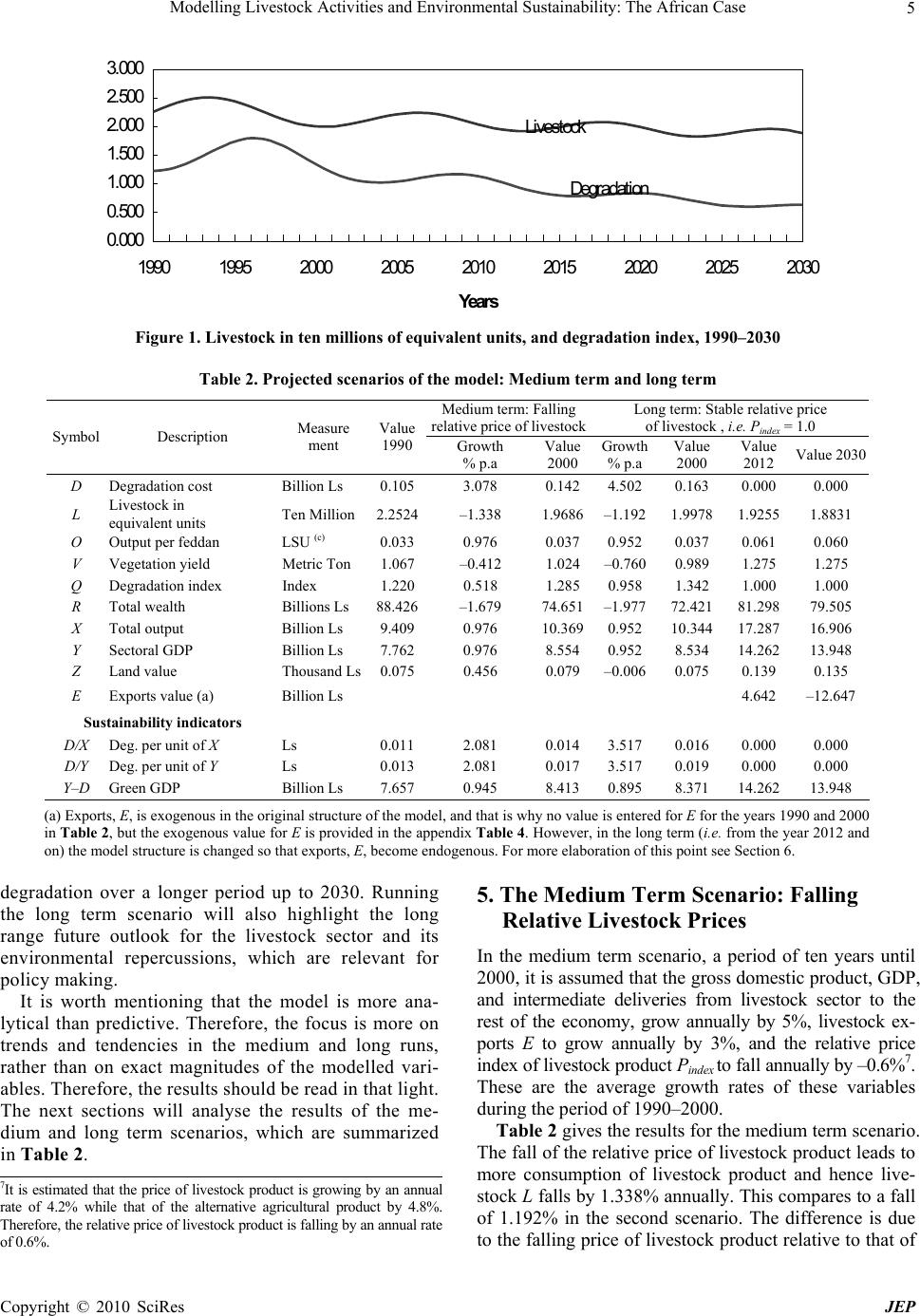

Modelling Livestock Activities and Environmental Sustainability: The African Case 5
0.000
0.500
1.000
1.500
2.000
2.500
3.000
1990 1995 2000 2005 2010 2015 2020 2025 2030
Years
Livestock
Degradation
Figure 1. Livestock in ten millions of equivalent units, and degradation index, 1990–2030
Table 2. Projected scenarios of the model: Medium term and long term
Medium term: Falling
relative price of livestock
Long term: Stable relative price
of livestock , i.e. Pindex = 1.0
Symbol Description Measure
ment
Value
1990 Growth
% p.a
Value
2000
Growth
% p.a
Value
2000
Value
2012 Value 2030
D Degradation cost Billion Ls 0.105 3.078 0.1424.502 0.163 0.000 0.000
L
Livestock in
equivalent units Ten Million 2.2524–1.338 1.9686–1.192 1.9978 1.9255 1.8831
O Output per feddan LSU (c) 0.033 0.976 0.0370.952 0.037 0.061 0.060
V Vegetation yield Metric Ton 1.067–0.412 1.024–0.7600.989 1.275 1.275
Q Degradation index Index 1.2200.518 1.2850.958 1.342 1.000 1.000
R Total wealth Billions Ls 88.426–1.679 74.651–1.97772.421 81.298 79.505
X Total output Billion Ls 9.4090.976 10.3690.952 10.344 17.287 16.906
Y Sectoral GDP Billion Ls 7.762 0.976 8.5540.952 8.534 14.262 13.948
Z Land value Thousand Ls0.0750.456 0.079–0.0060.075 0.139 0.135
E Exports value (a) Billion Ls 4.642 –12.647
Sustainability indicators
D/X Deg. per unit of X Ls 0.0112.081 0.0143.517 0.016 0.000 0.000
D/Y Deg. per unit of Y Ls 0.0132.081 0.0173.517 0.019 0.000 0.000
Y–D Green GDP Billion Ls 7.6570.945 8.4130.895 8.371 14.262 13.948
(a) Exports, E, is exogenous in the original structure of the model, and that is why no value is entered for E for the years 1990 and 2000
in Table 2, but the exogenous value for E is provided in the appendix Table 4. However, in the long term (i.e. from the year 2012 and
on) the model structure is changed so that exports, E, become endogenous. For more elaboration of this point see Section 6.
degradation over a longer period up to 2030. Running
the long term scenario will also highlight the long
range future outlook for the livestock sector and its
environmental repercussions, which are relevant for
policy making.
It is worth mentioning that the model is more ana-
lytical than predictive. Therefore, the focus is more on
trends and tendencies in the medium and long runs,
rather than on exact magnitudes of the modelled vari-
ables. Therefore, the results should be read in that light.
The next sections will analyse the results of the me-
dium and long term scenarios, which are summarized
in Table 2.
5. The Medium Term Scenario: Falling
Relative Livestock Prices
In the medium term scenario, a period of ten years until
2000, it is assumed that the gross domestic product, GDP,
and intermediate deliveries from livestock sector to the
rest of the economy, grow annually by 5%, livestock ex-
ports E to grow annually by 3%, and the relative price
index of livestock product Pindex
to fall annually by –0.6%7.
These are the average growth rates of these variables
during the period of 1990–2000.
Table 2 gives the results for the medium term scenario.
The fall of the relative price of livestock product leads to
more consumption of livestock product and hence live-
stock L falls by 1.338% annually. This compares to a fall
of 1.192% in the second scenario. The difference is due
to the falling price of livestock product relative to that of
7It is estimated that the price of livestock product is growing by an annual
rate of 4.2% while that of the alternative agricultural product by 4.8%.
Therefore, the relative price of livestock product is falling by an annual rate
of 0.6%.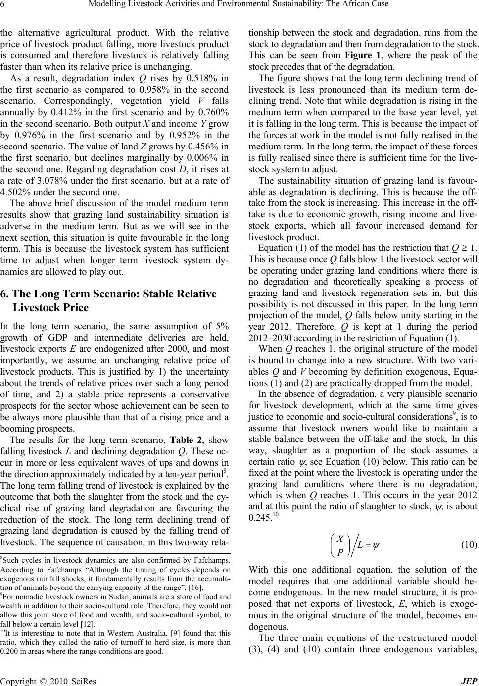

Modelling Livestock Activities and Environmental Sustainability: The African Case 6
the alternative agricultural product. With the relative
price of livestock product falling, more livestock product
is consumed and therefore livestock is relatively falling
faster than when its relative price is unchanging.
As a result, degradation index Q rises by 0.518% in
the first scenario as compared to 0.958% in the second
scenario. Correspondingly, vegetation yield V falls
annually by 0.412% in the first scenario and by 0.760%
in the second scenario. Both output X and income Y grow
by 0.976% in the first scenario and by 0.952% in the
second scenario. The value of land Z grows by 0.456% in
the first scenario, but declines marginally by 0.006% in
the second one. Regarding degradation cost D, it rises at
a rate of 3.078% under the first scenario, but at a rate of
4.502% under the second one.
The above brief discussion of the model medium term
results show that grazing land sustainability situation is
adverse in the medium term. But as we will see in the
next section, this situation is quite favourable in the long
term. This is because the livestock system has sufficient
time to adjust when longer term livestock system dy-
namics are allowed to play out.
6. The Long Term Scenario: Stable Relative
Livestock Price
In the long term scenario, the same assumption of 5%
growth of GDP and intermediate deliveries are held,
livestock exports E are endogenized after 2000, and most
importantly, we assume an unchanging relative price of
livestock products. This is justified by 1) the uncertainty
about the trends of relative prices over such a long period
of time, and 2) a stable price represents a conservative
prospects for the sector whose achievement can be seen to
be always more plausible than that of a rising price and a
booming prospects.
The results for the long term scenario, Table 2, show
falling livestock L and declining degradation Q. These oc-
cur in more or less equivalent waves of ups and downs in
the direction approximately indicated by a ten-year period8.
The long term falling trend of livestock is explained by the
outcome that both the slaughter from the stock and the cy-
clical rise of grazing land degradation are favouring the
reduction of the stock. The long term declining trend of
grazing land degradation is caused by the falling trend of
livestock. The sequence of causation, in this two-way rela-
tionship between the stock and degradation, runs from the
stock to degradation and then from degradation to the stock.
This can be seen from Figure 1, where the peak of the
stock precedes that of the degradation.
The figure shows that the long term declining trend of
livestock is less pronounced than its medium term de-
clining trend. Note that while degradation is rising in the
medium term when compared to the base year level, yet
it is falling in the long term. This is because the impact of
the forces at work in the model is not fully realised in the
medium term. In the long term, the impact of these forces
is fully realised since there is sufficient time for the live-
stock system to adjust.
The sustainability situation of grazing land is favour-
able as degradation is declining. This is because the off-
take from the stock is increasing. This increase in the off-
take is due to economic growth, rising income and live-
stock exports, which all favour increased demand for
livestock product.
Equation (1) of the model has the restriction that Q  1.
This is because once Q falls blow 1 the livestock sector will
be operating under grazing land conditions where there is
no degradation and theoretically speaking a process of
grazing land and livestock regeneration sets in, but this
possibility is not discussed in this paper. In the long term
projection of the model, Q falls below unity starting in the
year 2012. Therefore, Q is kept at 1 during the period
2012–2030 according to the restriction of Equation (1).
When Q reaches 1, the original structure of the model
is bound to change into a new structure. With two vari-
ables Q and V becoming by definition exogenous, Equa-
tions (1) and (2) are practically dropped from the model.
In the absence of degradation, a very plausible scenario
for livestock development, which at the same time gives
justice to economic and socio-cultural considerations9, is to
assume that livestock owners would like to maintain a
stable balance between the off-take and the stock. In this
way, slaughter as a proportion of the stock assumes a
certain ratio 
, see Equation (10) below. This ratio can be
fixed at the point where the livestock is operating under the
grazing land conditions where there is no degradation,
which is when Q reaches 1. This occurs in the year 2012
and at this point the ratio of slaughter to stock,  , is about
0.245.10
 





L
P
X (10)
With this one additional equation, the solution of the
model requires that one additional variable should be-
come endogenous. In the new model structure, it is pro-
posed that net exports of livestock, E, which is exoge-
nous in the original structure of the model, becomes en-
dogenous.
The three main equations of the restructured model
(3), (4) and (10) contain three endogenous variables,
8Such cycles in livestock dynamics are also confirmed by Fafchamps.
According to Fafchamps “Although the timing of cycles depends on
exogenous rainfall shocks, it fundamentally results from the accumula-
tion of animals beyond the carrying capacity of the range”, [16].
9For nomadic livestock owners in Sudan, animals are a store of food and
wealth in addition to their socio-cultural role. Therefore, they would no
t
allow this joint store of food and wealth, and socio-cultural symbol, to
fall below a certain level [12].
10It is interesting to note that in Western Australia, [9] found that this
ratio, which they called the ratio of turnoff to herd size, is more than
0.200 in areas where the range conditions are good.

Modelling Livestock Activities and Environmental Sustainability: The African Case 7
namely L, X and E. These equations are solved simul-
taneously and the results are used for solving the rest of
the model.
The solution of the endogenous variables under the
new structure of the model for the year 2012 and the year
2030 are presented in the last two columns of Table 2.
Note that livestock exports E are added to Table 2 as an
endogenous variable for the years 2012 and 2030. But
before the year 2012, E was exogenous and that is why it
is not shown in Table 2 before 2012. As can be seen
from the table, degradation cost D is zero in 2012 and
2030, since degradation index Q is unity in these two
years. The output X in 2030 is somewhat less than that in
2012. Therefore, the domestic output, which is used to
meet domestic consumption demand, is supplemented in
later years by imports of livestock product, i.e. net ex-
ports E < 0, see Table 2. This is explained by the out-
come that our assumption of unchanging relative price of
livestock product has ruled out any price adjustment
mechanism. Therefore, a quantity adjustment mechanism
has to adjust supply to rising demand, and the net exports
of livestock product E has to bear the burden of this ad-
justment, see Equation (4) of the model.
The above analysis shows that there are two adjust-
ment mechanisms at work in the long term. The first one
is internal to the livestock sector and the second one is
external. The internal one shows that the livestock
system is self-regulatory in the sense that it has a built-in
adjustment mechanism. This mechanism works through
the two-way relationship between the stock and
degradation. When the stock of grazing animals exceeds
grazing land carrying capacity degradation sets in. Due to
degradation the stock does not continue to grow steadily
and sustainably, since degradation adversely affects the
growth of the stock. After a certain point in time, the
stock is adjusted downward to the prevailing degradation
conditions on grazing land. The end result is that the
downward adjustment of the stock eases the pressure on
grazing land and hence degradation is mitigated.
The external adjustment mechanism originates from
the economic system and it works through economic
growth, foreign trade and relative prices. We have seen
the last one in the medium term analysis and in principle
it applies also for the long term11. Rising income, falling
relative price of livestock product and more livestock
exports lead to increasing off-take from the stock which
eases pressure on grazing land and ultimately reduces
degradation.
The results of the model suggest that it is possible to
reconcile the new range ecology thinking [4,17,19]
with that of the mainstream range management para-
digm. The latter, which assumes equilibrium12 envi-
ronment, argues that the number of animal population
is limited by availability of vegetation and the exis-
tence of excessive number of animals on the range ad-
versely affect vegetation and this leads in the long run
to rangeland degradation. The former, which assumes
disequilibrium environment, argue that both animal
population and vegetation are dominated by external
factors such as rainfall and animal population are kept
low by events such as drought and therefore animal
population cannot have long run adverse impact on
rangeland. The model results in the medium term seem
to confirm the mainstream range management thinking
while the model results in the long term seem to con-
firm the new range ecology thinking. Thus, whether
range ecology is in equilibrium or disequilibrium is not
a permanent situation but a situation that varies over
time. Therefore, it appears that both paradigms, equi-
librium and disequilibrium, have a grain of truth in
their views regarding the issue of land degradation.
7. More Discussion of Results
The lower part of Table 2 sums up several sustainability
indicators for the livestock sector. The sustainability
situation is relatively encouraging under the scenario of
changing relative prices as compared to the unchanging
one. Under the first scenario, degradation cost per unit of
output and value added, D/X and D/Y respectively, grow
by 2.081% per annum, compared to 3.517% under the
second scenario. Regarding the sectoral green GDP,
(Y–D), it grows by 0.945% under the first scenario and by
0.895% under second scenario. The concept of green
GDP here refers to the livestock sectoral GDP, Y, after
the deduction of the degradation cost of grazing land, D.
The degradation cost is supposed to be deposited in
separate fund for financing the reclamation of the
degraded land in the livestock sector, if production is to
be sustained into the future.
One important policy lesson which emerges from this
discussion is that a falling relative price of livestock
product encourages more consumption from the stock,
thereby eases the pressure on grazing land and ultimately
grazing land degradation is mitigated13. In other words,
subsidising the price of livestock product can be a policy
option for achieving sustainability in the livestock sector,
but this needs to be weighed against any distortionary
effects or fiscal problems that the subsidy may cause.
As an exercise in sensitivity analysis, the parameter 
11In the long term solution of the model and under changing relative
p
rices scenario (not reported here), the livestock system reaches the
p
oint of no degradation, i.e. Q =1, in much earlier time than under the
unchanging relative prices scenario, which we have seen here.
12The term (dis) equilibrium is used in ecology to refer to an ecosystem
where populations are in long term (im) balance with other elements o
f
the system [17].
13An IMF working paper shows that lower price of meat in Sudan leads
to more off-take from the stock since livestock owners want to supple-
ment their income and smooth consumption [18].

Modelling Livestock Activities and Environmental Sustainability: The African Case 8
that describes the final demand function for livestock
product has been increased by 5%. For some variables
such as the stock L and degradation index Q, the
projected trend has changed resulting in improved
sustainability of grazing land. This indicates that a shift
in consumers’ preferences towards more consumption
of livestock product promotes environmental sustain-
ability in the livestock sector.
Furthermore, an opportunistic management strategy
that involves an increase of vegetation yield V; effective
expansion of grazing land N; reduction of animals vege-
tation intake H; and reduction of the stock L can pre-
empt or reduce grazing land degradation, that is resulting
in lower Q.
8. Conclusions
Some important conclusions have emerged from the
analysis. First, the livestock system is dynamic and can
adjust when longer term system dynamics are allowed to
play out. Part of the adjustment mechanism is built in the
livestock system and the other part comes from the eco-
nomic system. The built-in adjustment mechanism works
through the two-way relationship between the stock and
degradation. The external adjustment mechanism, origi-
nating from the economic system, works through eco-
nomic growth, relative prices and foreign trade. Second,
although grazing land sustainability situation is favour-
able in the long term, yet it is adverse in the medium
term. Therefore, an external intervention in the form of
appropriate policies, that facilitate access to grazing land
and water, is needed to help the livestock system adjust
in the medium term and mitigate degradation. Also, op-
portunistic management strategy on the part of pastoral-
ists is an effective way of pre-empting and/or reducing
grazing land degradation. The model results seem to
suggest a reasonable synthesis of the traditional main-
stream range management approach with the new range
ecology thinking.
It is important to be reminded that the model is
more analytical than predictive. Its focus is more on
medium and long term trends rather than exact mang-
nitudes. Therefore its results should be understood in
that light.
REFERENCES
[1] L. R. Oldeman, R. T. A. Hakkeling, and W. G. Sombroek,
“World map of the status of human induced soil degradation:
An explanatory note,” ISRIC/UNEP, Wageningen, The
Netherlands, 1991.
[2] H. Dregne, M. Kassas, and B. Rozanov, “Status of deserti-
fication and implementation of United Nations plan to
combat desertification,” Desertification Control Bulletin, No.
20, pp. 6, 1991.
[3] C. de Haan, H. Steinfeld, and H. Blackburn, “Livestock and
the Environment: Finding a balance,” Study sponsored by
the European Commission, FAO and World Bank, 1997.
[4] I. Scoones, (Ed.) “Living under uncertainty: New directions
in pastoral development in Africa,” Intermediate Techno-
logy Publications, London, 1994.
[5] T. Amede, et al., “Maximizing benefits from livestock-
water venture in Sub-Saharan Africa: From concepts to
practices,” The International Water Management Institute/
International Livestock Research Institute, Addis Ababa,
Ethiopia, 2009.
[6] A. K. Acharya and N. Kafle, “Land degradation issues in
Nepal and its management: Through agroforestry,” The
Journal of Agriculture and Environment, Vol. 10, June 2009.
[7] A. de Sherbinin, “CIESIN thematic guide to land-use and
land-cover change,” Center for International Earth Science
Information Network (CIESIN), Columbia University,
Palisades, NY, USA, 2002.
[8] G. B. Thapa and G. S. Paudel, “Evaluation of the livestock
carrying capacity of land: Resources in the Hills of Nepal
based on total digestive nutrient analysis,” Agriculture,
Ecosystems & Environment, Vol. 78, No. 3, pp. 223–235,
May 2000.
[9] D. G. Wilcox and J. F. Thomas, “The Fitzroy valley
regeneration project in Western Australia,” in J. A. Dixon,
D. E. James and P. B. Sherman, Eds., “Dry management:
Economic case studies,” Earthscan Publications Ltd.,
London, 1990.
[10] L. C. Braat and J. B. Opschoor, “Risk in the Botswana
range-cattle system,” in J. A. Dixon, D. E. James and P. B.
Sherman, Eds., “Dry management: Economic case studies,”
Earthscan Publications Ltd., London 1990
[11] C. Berrings and D. I. Stern, “Modelling loss of resilience
in agroecosystems: Rangelands in Botswana,” Environ-
mental and Resource Economics, Vol. 16, No. 12, pp.
185–210, 2000.
[12] D. Pearce, E. Barbier, and A. Markandya, “Sustainable
development: Economics and environment in the Third
World,” Edward Elgar, England, 1990.
[13] A. R. Gigengack, C. J. Jepma, D. MacRae, and F. Poldy,
“Global modelling of dryland degradation,” in J. A. Dixon,
D. E. James and P. B. Sherman, Eds., “Dry management:
Economic case studies,” Earthscan Publications Ltd., Lon-
don, 1990.
[14] H. A. Simon, “Causal ordering and identifiability,” in W. C.
Hood and T. C. Koopmans, Eds., “Studies in econometric
method,” Cowles Foundation Monograph, No. 14, Yale
University Press, New Haven, 1953.
[15] E. Abdelgalil, “Economic policies for sustainable resource
development: Models applied to Sudan,” PhD thesis, Eras-
mus University Rotterdam, The Netherlands, 2000.
[16] M. Fafchamps, “The tragedy of the commons, livestock
cycles, and sustainability,” Journal of African Economies,
Vol. 7, No. 3, pp. 384–423, 1998.
[17] J. Ellis, “Climate variability and complex ecosystem dy-
namics: Implications for pastoral development,” in I.
Scoones, Ed., “Living under uncertainty: New directions in
pastoral development in Africa,” Intermediate Technology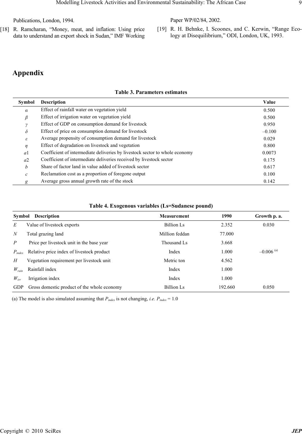

Modelling Livestock Activities and Environmental Sustainability: The African Case 9
Publications, London, 1994.
[18] R. Ramcharan, “Money, meat, and inflation: Using price
data to understand an export shock in Sudan,” IMF Working
Paper WP/02/84, 2002.
[19] R. H. Behnke, I. Scoones, and C. Kerwin, “Range Eco-
logy at Disequilibrium,” ODI, London, UK, 1993.
Appendix
Table 3. Parameters estimates
Symbol Description Value
α Effect of rainfall water on vegetation yield 0.500
β Effect of irrigation water on vegetation yield 0.500
γ Effect of GDP on consumption demand for livestock 0.950
δ Effect of price on consumption demand for livestock –0.100
ε Average propensity of consumption demand for livestock 0.029
η Effect of degradation on livestock and vegetation 0.800
a1 Coefficient of intermediate deliveries by livestock sector to whole economy 0.0073
a2 Coefficient of intermediate deliveries received by livestock sector 0.175
b Share of factor land in value added of livestock sector 0.617
c Reclamation cost as a proportion of foregone output 0.100
g Average gross annual growth rate of the stock 0.142
Table 4. Exogenous variables (Ls=Sudanese pound)
Symbol Description Measurement 1990 Growth p. a.
E Value of livestock exports Billion Ls 2.352 0.030
N Total grazing land Million feddan 77.000
P Price per livestock unit in the base year Thousand Ls 3.668
Pindex Relative price index of livestock product Index 1.000 –0.006 (a)
H Vegetation requirement per livestock unit Metric ton 4.562
Wrain Rainfall index Index 1.000
Wirr Irrigation index Index 1.000
GDP Gross domestic product of the whole economy Billion Ls 192.660 0.050
(a) The model is also simulated assuming that Pindex is not changing, i.e. Pindex = 1.0