Journal of Biomedical Science and Engineering
Vol. 5 No. 12A (2012) , Article ID: 26264 , 9 pages DOI:10.4236/jbise.2012.512A109
A wavelet-based super-resolution method for multi-slice MRI
![]()
1School of Engineering and Information Technology (SEIT), University of New South Wales, Canberra, Australia
2The Trauma and Orthopaedic Research Unit, The Canberra Hospital, Canberra, Australia
Email: Rafiqul.Islam@student.adfa.edu.au, a.lambert@adfa.edu.au, M.Pickering@adfa.edu.au
Received 4 November 2012; revised 7 December 2012; accepted 16 December 2012
Keywords: Magnetic Resonance Imaging; Super Resolution; Gaussian Scale Mixture Model; Wavelet Regularization
ABSTRACT
In multi-slice magnetic resonance imaging (MRI), the resolution in the slice direction is usually reduced to allow faster acquisition times and to reduce the amount of noise in each 2D slice. To address this issue, a number of super resolution (SR) methods have been proposed to improve the resolution of 3D MRI volumes. Most of the methods involve the use of prior models of the MRI data as regularization terms in an ill-conditioned inverse problem. The use of user-defined parameters produces better results for these approaches but an inappropriate choice may reduce the overall performance of the algorithm. In this paper, we present a wavelet domain SR method which uses a Gaussian scale mixture (GSM) model in a sparseness constraint to regularize the ill-posed SR inverse problem. The proposed approach also makes use of an extension of the Dual Tree Complex Wavelet Transform to provide the ability to analyze the wavelet coefficients with sub-level precision. Our results show that the 3D MRI volumes reconstructed using this approach have quality superior to volumes produced by the best previously proposed approaches.
1. INTRODUCTION
Magnetic resonance imaging (MRI) is an imaging technique for producing images of parts of the human body for clinical purposes. When compared to other widely used scanning methods such as Computed Tomography (CT) and Positron Emission Tomography (PET), MRI has the advantage of using only strong magnetic fields and non-ionizing radiation in the radio frequency range. In multi-slice MRI, multiple 2D slices are captured to form a 3D volume of the desired body part. Recently, faster multi-slice acquisition methods (such as Single-shot Spin Echo, Conventional Spin Echo, etc.) are often used to capture MRI slices in the presence of motion of the imaging subjects [1,2]. During this faster acquisition, high-resolution image slices are obtained in the in-plane direction but some undesirable artifacts are observed due to the resolution reduction in the slice-select direction [3]. As a result of this resolution reduction, some valuable information may be lost [4]. To deal with this problem, a number of image super resolution (SR) techniques have been used as post-processing methods to improve the quality of the low-resolution images [5].
The basic idea underlying all SR algorithms is the combination of a number of low-resolution (LR) blurred noisy images to produce an SR image [6]. Within this wide area of study, medical image super resolution has emerged as a particularly active field and initial attempts at the application of SR reconstruction algorithms for MRI images were made in [7,8]. In [7], the authors utilized an iterative back projection (IBP) method [9] to improve the in-plane resolution of diffusion-weighted images. In their method, the low resolution images were acquired by sub-pixel shifting in the phase-encode and frequency-encode direction. Since each of the sub-pixel shifted images contained identical information but with different noise [10,11] a small improvement in resolution can be obtained. In [8] the authors improved this method by utilizing sub-pixel shifts in the slice-select direction instead of in the in-plane direction during the multi-slice acquisition. In their work, a number of multi-slice low resolution volumes were acquired where each volume was shifted with respect to the other volumes by a subpixel amount in the slice-select direction. These multiple parallel overlapping slice stacks were combined using their proposed super resolution reconstruction algorithm to produce a 3D isotropic volume with improved resolution and sharper edges in the slice-select direction. The authors in [12,13] also utilized the IBP reconstruction method to improve the resolution in the sliceselect direction. However, the blur and sharpening kernel used in their approach introduced some unwanted noise and artifacts. The SR method proposed in [13] was more effective in improving the slice-select direction resolution as a more appropriate blur kernel was utilized.
More recently, the use of regularization prior models has improved the performance of SR algorithms. An SR reconstruction technique based on the use of a discontinuity-preserving regularization method was proposed in [14] The authors demonstrated that an SR approach using this priori model increased the ability of clinicians to detect and visualize small regions of neuronal activity. Moreover, the activated regions appeared sharper and provided better information regarding their morphological limits and structure. Shantanu et al. [15] proposed an MRI resolution enhancement algorithm that made use of a total variation (TV) prior. They also utilized an edgepreserving operator during the up-sampling and downsampling of images that enhanced the spatial resolution. Recently, a spatial-domain regularization approach for SR was proposed in [16]. This regularization method, known as directional bilateral total variation (DBTV), applied a directionally adaptive weighting on the traditional total variation regularization approach. Schilling et al. introduced a multi-stack approach in [17] where a number of LR MRI volumes were captured at different orientations and combined to produce an SR volume using the simultaneous additive reconstruction technique (SART). They showed that capturing the LR images at different orientations produced superior results than when using a parallel stack approach [8] where the LR images were captured at different distances along the slice-select direction only.
In this paper, we address the problem of choosing an appropriate regularization prior model in SR reconstruction methods to improve the resolution of MRI volumes in the slice-select direction. In [18], we demonstrated the benefits of using a GSM model of a standard wavelet transform as a prior for simulated MRI data. In the approach presented here we adopt an extended waveletdomain regularization prior model to analyze the wavelet coefficients with sub-level precision. Our experimental results for both simulated and real MRI data show that this algorithm produces SR volumes with quality superior to volumes produced by the best previously proposed approaches.
The remainder of the paper is organized as follows: In Section 2, we explain the concept of our sub-level wavelet transform. The general approaches used for SR are described in Section 3 and our proposed extensions to this approach for generating a super-resolution volume are presented in Section 4. Section 5 is devoted to describing the experimental evaluation of the algorithms and finally our conclusions are presented in Section 6.
2. THE SUB-LEVEL WAVELET TRANSFORM
The wavelet transform has been widely used as a multiresolution data analysis method across the field of signal processing for applications such as image denoising, image de-blurring and image enhancement. The DTCWT, originally introduced by Kingsbury in [19] has been shown to be a superior wavelet transform in the field of image processing because of its shift invariant and directionally oriented properties. In general, the wavelet transform of an image x can be expressed as follows:
 (1)
(1)
where Wj represents the wavelet transform operation and ψj are the wavelet coefficients for scale levels j = 1, 2 ××× L.
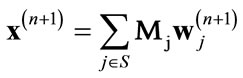
In this paper, we extend the DTCWT by adding an extra level in between each traditional level. This extra level provides more information during the subsequent analysis of the images. The new wavelet transform of an image x is implemented by adding an extra level and the overall operation of this transformation can be described as follows: Firstly the normal DTCWT is calculated as in Eq.1. Then to add an extra level, we resize the original volume by a factor of 2–0.5 using linear interpolation and apply the wavelet transform again. This transformation produces wavelet coefficients for scale levels j = 1.5, 2.5 ××× L + 0.5. Finally, we merge these two sets of wavelet coefficients to produce the new wavelet coefficients for scale levels j = 1, 1.5, 2 ××× L, L + 0.5. These extended set of coefficients effectively have sub-level resolution and provide the ability to better analyze the inter-level relationships between coefficients during the component wise de-noising stage of our proposed SR framework. The overall sub-level wavelet decomposition process using the above process is illustrated in Figure 1.
3. BACKGROUND
The main objective of image deconvolution algorithms is to find the solution of an ill-conditioned equation of the form:
 (2)
(2)
where x0 is a vector of pixel values from the original image, y is a vector of pixel values from the observed blurry image, H represents a convolution (i.e. blockcirculant) matrix that approximates the blurring function and b is a vector representing white noise with zero mean and variance σ2 [20].
A solution to this minimization problem can be ex-
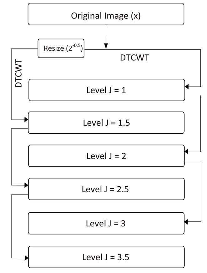
Figure 1. Flowchart for a 3 level wavelet decomposition with an extra tree based on a resized image.
plained by first considering the case when the noise term b is set to zero. The cost function for this case is given by:
 (3)
(3)
The solution that minimizes this cost function is given by the gradient descent method as follows:
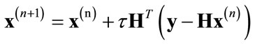 (4)
(4)
where τ is a fixed step size and HT represents the backprojection kernel that should be the pseudo-inverse of the convolution matrix. This equation represents the classic Landweber iteration [21].
Daubechies et al. proposed a solution to the problem of estimating the value of x0 when both blurring and noise are present by using the thresholded-Landweber algorithm [22]. This approach consists of first performing the Landweber iteration with step-size τ:
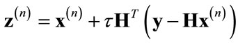 (5)
(5)
and then performing the wavelet domain de-noising operation:
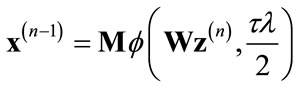 (6)
(6)
The function f(w,t) is the soft-thresholding function defined in [22,23] with the form:
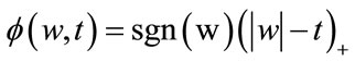 (7)
(7)
where (.)+ is the positive-part function given by:
 (8)
(8)
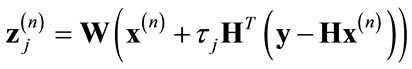
Vonesch and Unser [23] improved this approach by developing the fast thresholded-Landweber (FTL) deblurring algorithm. In their approach, the original thresholded-Landweber operation is performed on a wavelet sub-band basis using different step-sizes for each subband as follows: For each sub-band j, perform the Landweber iteration:
 (9)
(9)
where Wj represents the wavelet transform operation for sub-band j, τj = 1/αj and αj is the sub-band emphasis factor defined in [23]. Then perform the wavelet domain soft-thresholding de-noising operation on each sub-band and apply the inverse wavelet transform to find the updated version of x as follows:
 (10)
(10)
where Mj represents the inverse wavelet transform operation for sub-band j.
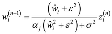
Zhang and Kingsbury [24] extended this algorithm by utilizing the element wise de-noising operation on each sub-band instead of the soft-thresholding de-noising function. The de-noising operation for every element in the sub-band j is given by
 (11)
(11)
where wj and zj are coefficients in the sub-band j, wt is calculated using the bivariate shrinkage de-noising algorithm defined in [25] on the wavelet coefficients of x(n), σ2 is the variance of measurement noise and ε is a stabilizer to avoid infinity. An inverse wavelet transform is then used to find the new estimate.
 (12)
(12)
This de-noising approach was shown by Zhang and Kingsbury in [24] to be equivalent to replacing the l1 norm sparseness constraint with a sparseness constraint that is closer to the l0 norm.
4. SUPER RESOLUTION USING A GSM MODEL CONSTRAINT
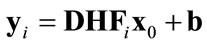
The resolution of any image is dependent on the properties of the sensors in the imaging device. Hence, the objective of a super resolution algorithm is to find the solution of an ill-conditioned equation of the form:
 (13)
(13)
where yi is a vector of pixel values from the ith observed image, Fi is a warping matrix, D is a sub-sampling matrix and bi represents the noise.
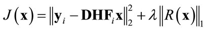
Since estimating x0 given yi is an ill-posed inverse problem, it is necessary to rely on prior information about the original signal to obtain an accurate estimate with robustness to noise. Including this prior information results in a minimization problem where the quality of a given estimate x is measured by a cost function of the form:
 (14)
(14)
The first term in this cost function quantifies the error between the observed LR image yi and an estimate of yi calculated from the current estimated high resolution image x. The second term is designed to penalize the estimated image when it does not conform to the prior model and thus helps to obtain a stable solution. The regularization parameter λ balances the contribution of both terms. The super resolution problem now becomes one of finding an estimate x of the original higher resolution image that minimizes the cost function J(x).
In this paper, for the regularization prior model, we use the wavelet domain GSM model as well as the sublevel wavelet domain GSM model. The main benefits of GSM model is it has the ability to regularize the estimated MRI volumes in terms of both the heavy tail distributions and the inter-scale properties of wavelet coefficients [26,27].
In our proposed wavelet domain GSM method, we extend the modified FTL algorithm to include multiple observed images and sub-sampling in the image acquisition model. To accommodate this extension, we modify the Landweber iteration as follows:
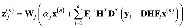 (15)
(15)
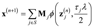
where  is the inverse of the warping operator and DT is an up-sampling matrix. A component-wise wavelet based de-noising operation is then performed on every sub-band j and the inverse wavelet transform is applied to find the updated version of x using Eq.12.
For our proposed sub-level wavelet domain GSM method, we use the extension of the DTCWT instead of the normal DTCWT discussed in Section 2 as a wavelet transform. The main benefit of this model over the normal GSM model is that it provides the ability to analyze the inter-level relationships between sub-level wavelet coefficients with finer resolution.
The algorithm starts with an initial guess of the highresolution image x from a set of low-resolution images. In our work, we choose one reference volume and used the cubic interpolation approach to create the initial highresolution image. Then an iterative process is used by alternating between the new modified Landweber iteration and de-noising method to estimate the output. The overall procedure is summarized in Figure 2.
5. PERFORMANCE EVALUATION
Experiments were conducted to evaluate the performance of the proposed SR algorithm for the purposes of increasing the resolution of 3D MRI volumes. We compared the performance of our proposed algorithm with a SR algorithm based on DBTV [16] as well as the SART approach [17] as these were found to be the best performing of the recently proposed SR approaches. The wavelet transform we have used in our proposed algorithm is a 3D version of the DTCWT. In the MRI acquisition process, the point spread function (PSF) is defined by the slice excitation profile function. In our experiment, we assume the slice profile function is approximated by a Gaussian function with the full-width half maximum (FWHM) distance set to the selected slice thickness.
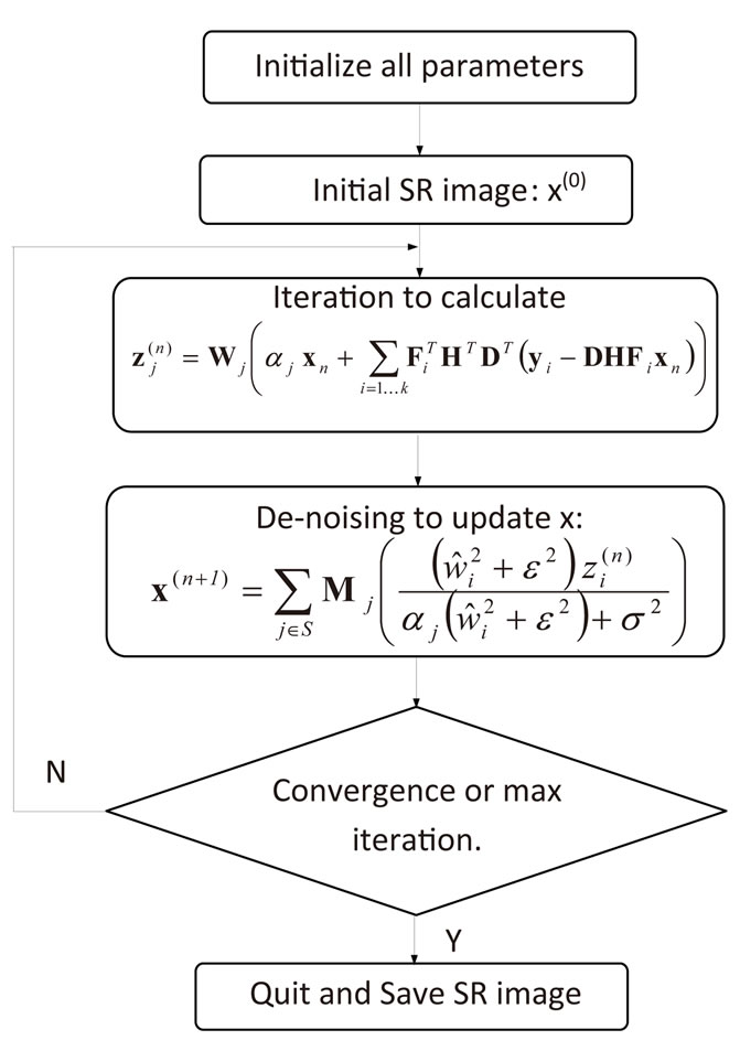
Figure 2. Flowchart for our proposed SR algorithm.
5.1. Volume Reconstruction Using Simulated Data
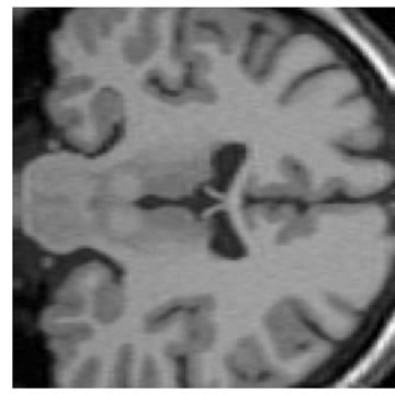
The input data used was a 3D MRI volume from the Brain Web Simulated Database [28]. Figure 3(a) shows a slice from the original volume. In our experiment, we took a 3D volume with 1 mm voxel resolution in the slice-select direction. We simulated the low-resolution volumes by rotating the original volume about all three axes simultaneously by 1, 2, 3 and 4 degrees. Each of these rotated volumes was then sub-sampled by a factor of 4 in the slice-select direction. Blur and noise were also added to simulate the effect of the image acquisition process. We used the multi-stack approach of capturing the LR volume at different orientations as this technique was shown in [17] to give better performance than the parallel stack approach. Figure 3(b) shows a slice from one of the sub-sampled, blurred and noisy input volumes, Figure 3(c) shows one slice from the output volume of the SR with DBTV algorithm, Figure 3(d) shows one slice from the output volume of the SR algorithm using SART, Figure 3(e) shows one slice from the output volume of our proposed SR algorithm using a GSM model prior [18] and Figure 3(f) shows one slice from the output volume of our proposed SR algorithm which incorporates both a GSM model prior and the sub-level wavelet transform described in Section 4. These images clearly show the improved subjective quality of the output of our proposed approach. The arrows in Figure 3(f) indicate example areas of improved resolution for the proposed algorithm.
For a practical measure of the quality of the estimated super resolution volume, we use a measure of the accuracy of a 3D segmented region produced using the estimated volumes. We call this measure the segmentation difference (SD) and it is defined as the percentage of voxels which are segmented differently for the estimated volume compared to the original volume. We use the formulae below to define SD.
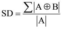 (16)
(16)
where A is a binary volume created by segmenting the SR volume and B is a binary volume created from the original volume. In order to create these segmented binary volumes, a thresholding technique is applied to the estimated super resolution volume and the original volume. This can be expressed as
 (17)
(17)
where T is the threshold value.
For a more standard evaluation, we compared the peak
 (a)
(a)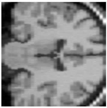 (b)
(b)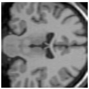 (c)
(c)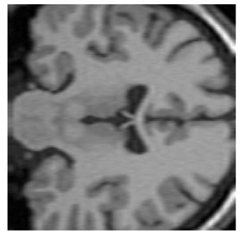 (d)
(d)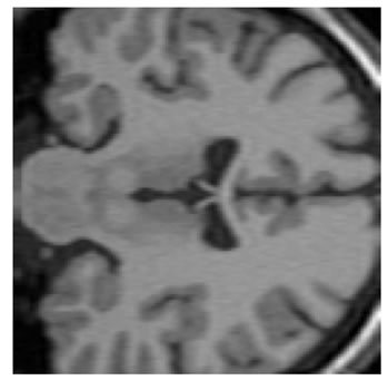 (e)
(e)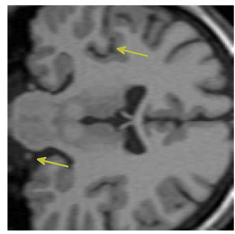 (f)
(f)
Figure 3. One slice from (a) The original volume, Original Slice; (b) One of the LR input volumes, Low resolution slice; (c) The output volume for the SR with DBTV algorithm, SR with DBTV; (d) The output volume from the SR with SART algorithm, SR with SART; (e) The output volume for the proposed SR with GSM constraint algorithm, Proposed GSM method; (f) The output volume for the proposed SR with sub-level GSM constraint algorithm, Proposed sub-level GSM method.
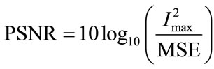
signal to noise ratio (PSNR) between the output volume and the original volume as a function of the iteration number. We use the following formula to define the PSNR.
 (18)
(18)
where Imax is the highest possible intensity value of the image volume and MSE is the mean squared error between the original volume and the output of the SR volume.
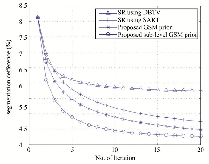
The results using these measurements for all algorithms are shown in Figure 4 and Table 1. Figure 4(a) shows a plot of the SD as a percentage at each iteration when the white matter from the estimated SR volumes was segmented and compared to the segmented white matter from the original volume. Figure 4(b) shows the curves for PSNR of the estimated volume compared to the original volume for each SR technique. These results show that the performance of both our proposed SR algorithms which use a GSM constraint are superior to the alternative SR with DBTV and SR with SART algorithms and the sub-level GSM approach provides improved performance over the algorithm which uses the standard DTCWT. The PSNR values when compared with the original volume after the final iterations of each algorithm are shown in Table 1. The results in Figures 3 and 4 and Table 1 clearly show the superior resolution improvement for this type of data when using our proposed methods.
5.2. Volume Reconstruction Using Real MRI Data
For a more practical evaluation, we tested our algorithm by using four sets of real knee MRI data of size 256 × 256 × 64 pixels. The slice thickness of each low-resolution volume was 2 mm and the in-plane resolution was 0.7 mm × 0.7 mm. The four data volumes used in our experiment were taken at different orientations. 3D rigid body registration was applied to align the femur in all four LR volumes. We then applied our proposed algorithm as well as the other algorithms described in the previous section to recover an SR volume from the set of LR volumes.
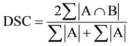
It is difficult to show quantitatively that SR has been achieved for real LR MRI data volumes. In this paper we chose to compare the shape of the segmented bones from the SR MRI volumes to the shape of the segmented bone from a CT volume of the same knee. Again we use the SD as defined in Section 5.1 as well as the dice similarity coefficient (DSC) as defined below:
 (19)
(19)
 (a)
(a)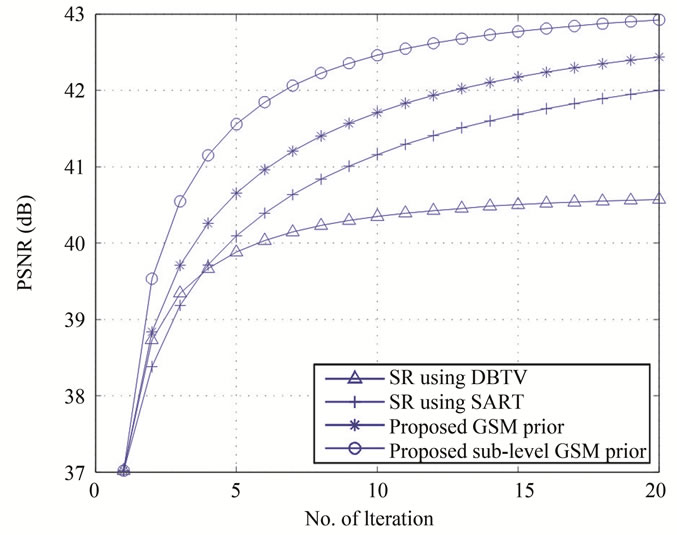 (b)
(b)
Figure 4. (a) The segmentation difference and (b) The PSNR for the SR algorithms using DBTV, SART and the proposed GSM and sub-level GSM model constraints.
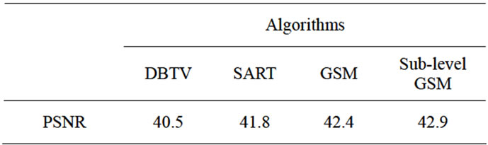
Table 1. Final PSNR values for each algorithm (dB).
The DSC determines the degree of overlap between the segmented output of the SR MRI volumes and the segmented CT volume. A higher value for the DSC measure indicates more similarity between two segmented volumes.
The slice thickness for the CT scan was 0.5 mm and the in-plane resolution was 0.335 mm × 0.335 mm. We then segmented the femur from the CT volume and from the SR MRI volume. It is difficult to segment the MRI femur using a fully automated segmentation algorithm because of noise and more than one tissue type in the MRI volume. Therefore the application of manual preprocessing steps were required to properly segment the output of the SR MRI volumes. The output slices of the SR MRI volumes were first manually delineated to select the boundary of the femur. An automated segmentation algorithm was then utilized to properly extract the femur from the semi-segmented SR MRI volumes. Finally a 3D multi-modal image registration method was applied to align the segmented bone from the CT volume and the segmented bone from the output of the SR MRI volumes. In our work, we used a 3D version of the inverse compositional algorithm [29] for image registration. The sum of conditional variance was used as the similarity measure instead of the sum of square difference as it has been shown to provide good results for multi-modal image registration [30]. Before the registration, we calibrated the CT image with the output of the SR MRI volume so that both image volumes were at the same scale. The SD and DSC measures were then calculated using the registered segmented femur from the SR MRI volumes and CT volume. The results for SD and DSC expressed as a percentage are shown in Table 2.
For a final analysis and evaluation, we measured the standard deviation of the difference between the surface of the segmented bone in the CT volume and the surface of the bone in the output of the SR MRI volumes. The lower the standard deviation, the more closely the surface of the bone reconstructed from the MRI matches the surface obtained from the CT volume. The standard deviation of the surface distances between these two modalities is shown in Table 3.
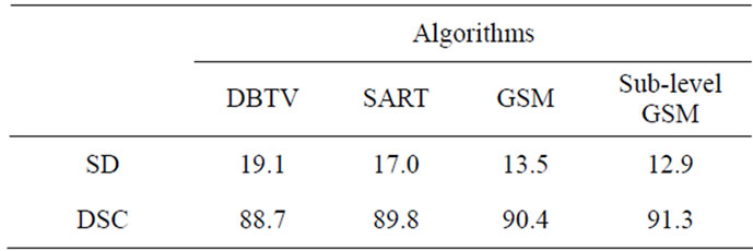
Table 2. Final SD and DSC values for each Algorithm (%).
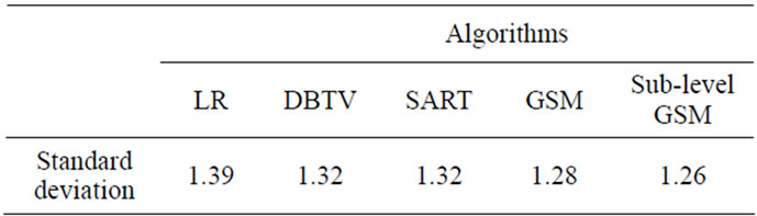
Table 3. Standard deviation of the distance between the surfaces of the femur segmented from the CT and the LR and SR MRI volumes (mm).
 (a)
(a)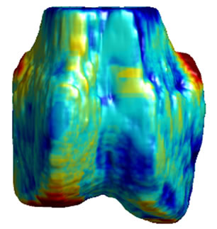 (b)
(b)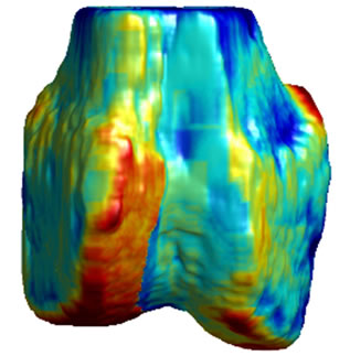 (c)
(c)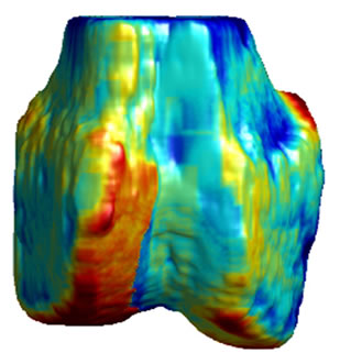 (d)
(d)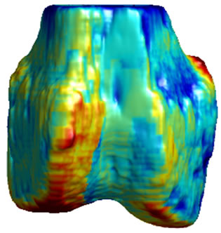 (e)
(e)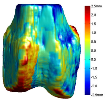 (f)
(f)
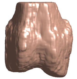
Figure 5. 3D surface renderings of the femur derived from (a) the segmented CT volume, CT Surface; (b) One of the LR MRI volumes, Low resolution volume; (c) The output volume for the SR with DBTV algorithm, SR with DBTV; (d) The output volume from the SR with SART algorithm, SR with SART; (e) The output volume for the proposed SR with GSM constraint algorithm, Proposed GSM method; (f) The output volume for the proposed SR with sub-level GSM constraint algorithm Proposed sub-level GSM method. The surface colours in (b)-(f) indicate the distance in millimeters between the surface derived from the CT volume in (a) and those obtained from the different MRI volumes.
Figure 5(a) shows a single-colour 3D rendering of the surface of the femur derived from the segmented CT volume. Figures 5 (b)-(f) show 3D renderings of the same CT surface but with colours used to illustrate the distance from the bone surface derived from the CT volume to the bone surfaces derived from the different MRI volumes. The colourbar in Figure 5(f) indicates the distance in millimeters that corresponds to each colour. Figures 5(b)-(f) show the distances between the surface derived from the CT volume and the surface derived from the LR input volume, the output of the SR algorithm using DBTV, the output of the SR algorithm using SART, the output of our proposed SR algorithm using a GSM constraint and the output of our proposed SR algorithm using a sub-level wavelet transform and a GSM constraint respectively. Although there is some residual difference in the surfaces produced by the MRI and CT volumes, these surface renderings show the improvement provided by the proposed GSM model constraint and further improvement provided by using the sub-level wavelet transform.
6. CONCLUSION
In this paper, we have presented a novel SR algorithm where a sub-level wavelet transform is incorporated with the use of a GSM model wavelet sparseness constraint. The algorithm takes several multi-slice volumes of the same anatomical region captured at different orientations and combines these low-resolution volumes together to form a single 3D volume with much higher resolution in the slice-select direction. We have tested our algorithm using both synthetic and real MRI data both visually and quantitatively. From these error measurements, we can conclude that the proposed approaches provide a superior improvement in resolution when compared to the best performing previously proposed approaches.
REFERENCES
- Huppert, B.J., Brandt, K.R., Ramin, K.D. and King, B.F. (1999) Single-shot fast spin-echo MR imaging of the Fetus: A pictorial essay. Radiographics, 19, 215-227. http: //radiographics.rsna.org/content/19/suppl 1/S215
- Vignaux, O.B., et al. (2001) Comparison of single-shot fast spin-echo and conventional spin-echo sequences for MR imaging of the heart: Initial experience. Radiology, 219, 545-550. http://radiology.rsna.org/content/219/2/545
- Gholipour, A., Estroff, J. and Warfield, S. (2010) Robust super-resolution volume reconstruction from slice acquisitions: Application to fetal brain MRI. IEEE Transactions on Medical Imaging, 29, 1739-1758. doi:10.1109/TMI.2010.2051680
- Greenspan, H. (2009) Super-resolution in medical imaging. The Computer Journal, 52, 43-63 doi:10.1093/comjnl/bxm075
- Plenge, E., et al. (2012) Super-resolution methods in MRI: Can they improve the trade-off between resolution, signal-to-noise ratio, and acquisition time? Magnetic Resonance in Medicine, 68, 1983-1993. doi:10.1002/mrm.24187
- Park, S.C., Park, M.K. and Kang M.G. (2003) Superresolution image reconstruction: A technical overview. IEEE Signal Processing Magazine, 20, 21-36. doi:10.1109/MSP.2003.1203207
- Peled, S. and Yeshurun, Y. (2001) Super resolution in MRI: Application to human white matter fiber tract visualization by diffusion tensor imaging. Magnetic Resonance in Medicine, 45, 29-35. doi:10.1002/1522-2594(200101)45:1<29::AID-MRM1005>3.0.CO;2-Z
- Greenspan, H., Peled, S., Oz, G. and Kiryati N. (2001) MRI inter-slice reconstruction using super-resolution. Prceedings of Medical Image Computing and ComputerAssisted Intervention MICCAI 2001, Lecture Notes in Computer Science, 2208, 1204-1206.
- Irani, M. and Peleg, S. (1991) Improving resolution by image registration. CVGIP: Graphical Models and Image Processing, 53, 231-239. doi:10.1016/1049-9652(91)90045-L
- Scheffler, K. (2002) Superresolution in MRI? Magnetic Resonance in Medicine, 48, 408-408. doi:10.1002/mrm.10203
- Kramer, D., et al. (1990) Applications of voxel shifting in magnetic resonance imaging. Investigative Radiology, 25, 1305-1310. doi:10.1097/00004424-199012000-00006
- Greenspan, H., Oz, G., Kiryati, N. and Peled, S. (2002) Super-resolution in MRI. Proceedings of the IEEE International Symposium on Biomedical Imaging, Washington DC, 7-10 July 2002, 943-946. doi:10.1109/ISBI.2002.1029417
- Yan, Z. and Lu, Y. (2009) Super resolution of MRI using improved IBP. Proceedings International Conference on Computational Intelligence and Security, Beijing, 11-14 December, 643-647.
- Peeters, R.R., et al. (2004) The use of super-resolution techniques to reduce slice thickness in functional MRI. International Journal of Imaging Systems and Technology, 14, 131-138. doi:10.1002/ima.20016
- Joshi, S., et al. (2009) MRI resolution enhancement using total variation regularization. Proceedings IEEE International Symposium on Biomedical Imaging: From Nano to Macro, Boston, 28 June - 1 July 2009, 161-164.
- Ben-Ezra, A., Greenspan, H. and Rubner Y. (2009) Regularized super-resolution of brain MRI. Proceedings IEEE International Symposium on Biomedical Imaging: From Nano to Macro, Boston, 28 June - 1 July 2009, 254-257.
- Shilling, R., et al. (2009) A super-resolution framework for 3-D high-resolution and high-contrast imaging using 2-D multi-slice MRI. IEEE Transactions on Medical Imaging, 28, 633-644. doi:10.1109/TMI.2008.2007348
- Islam, R., Lambert, A.J. and Pickering, M.R. (2012) Super resolution of 3D MRI images using a Gaussian scale mixture model constraint. Proceedings IEEE International Conference on Acoustics, Speech and Signal Processing, Kyoto, 25-30 March 2012, 849-852.
- Kingsbury, N. (2001) Complex wavelets for shift invariant analysis and filtering of signals. Applied and Computational Harmonic Analysis, 10, 234-253. doi:10.1006/acha.2000.0343
- Bertero, M. and Boccacci, P. (1998) Introduction to inverse problems in imaging. Taylor & Francis, Bristol. doi:10.1887/0750304359
- Landweber, L. (1951) An iteration formula for fredholm integral equations of the first kind. American Journal of Mathematics, 73, 615-624. doi:10.2307/2372313
- Daubechies, I., Defrise, M. and De Mol, C. (2004) An iterative thresholding algorithm for linear inverse problems with a sparsity constraint. Communications on Pure and Applied Mathematics, 57, 1413-1457. doi:10.1002/cpa.20042
- Vonesch, C. and Unser, M. (2008) A fast thresholded landweber algorithm for wavelet-regularized multidimensional de-convolution. IEEE Transactions on Image Processing, 17, 539-549. doi:10.1109/TIP.2008.917103
- Zhang, Y. and Kingsbury, N. (2009) Image deconvolution using a Gaussian Scale Mixtures model to approximate the wavelet sparseness constraint. Proceedings of IEEE International Conference on Acoustics, Speech and Signal Processing, Taipei, 19-24 April 2009, 681-684. doi:10.1109/ICASSP.2009.4959675
- Sendur, L. and Selesnick, I. (2002) Bivariate shrinkage functions for wavelet-based denoising exploiting interscale dependency. IEEE Transactions on Signal Processing, 50, 2744-2756. doi:10.1109/TSP.2002.804091
- Andrews, D.F. and Mallows, C.L. (1974) Scale mixtures of normal distributions. Journal of the Royal Statistical Society. Series B (Methodological), 36, 99-102. http://www.jstor.org/stable/2984774
- Wainwright, M.J. and Simoncelli, E.P. (2000) Scale mixtures of Gaussians and the statistics of natural images. Advanced Neural Information Processing Systems, 12, 855-861.
- Collins, D., et al. (1998) Design and construction of a realistic digital brain phantom. IEEE Transactions on Medical Imaging, 17, 463-468. doi:10.1109/42.712135
- Baker, S. and Matthews, I. (2004) Lucas-Kanade 20 years on: A unifying framework. International Journal of Computer Vision, 56, 221-255. doi:10.1023/B:VISI.0000011205.11775.fd
- Pickering, M.R. (2011) A new similarity measure for multi-modal image registration. Proceedings of IEEE International Conference on Image Processing, Brussels, 11-14 September, 2011, 2273-2276.