Engineering
Vol. 3 No. 4 (2011) , Article ID: 4603 , 4 pages DOI:10.4236/eng.2011.34049
Application of Least Square Support Vector Machine (LSSVM) for Determination of Evaporation Losses in Reservoirs
Centre for Disaster Mitigation and Management, VIT University, Vellore, India
E-mail: pijush.phd@gmail.com
Received November 5, 2010; revised December 8, 2010; accepted December 13, 2010
Keywords: Evaporation Losses, Least Square Support Vector Machine, Prediction, Artificial Neural Network
ABSTRACT
This article adopts Least Square Support Vector Machine (LSSVM) for prediction of Evaporation Losses (EL) in reservoirs. LSSVM is firmly based on the theory of statistical learning, uses regression technique. The input of LSSVM model is Mean air temperature (T) (˚C), Average wind speed (WS) (m/sec), Sunshine hours (SH) (hrs/day), and Mean relative humidity (RH) (%). LSSVM has been used to compute error barn of predicted data. An equation has been developed for the determination of EL. Sensitivity analysis has been also performed to investigate the importance of each of the input parameters. A comparative study has been presented between LSSVM and artificial neural network (ANN) models. This study shows that LSSVM is a powerful tool for determination EL in reservoirs.
1. Introduction
One of the most effective water loss processes of reservoir is the evaporation. The amount of evaporation occurs often in large quantities. For example, in late 1950s total evaporation from water surfaces in the United States was greater than the total amount of water withdrawn for domestic purposes by cities and towns [1]. Therefore, the determination of Evaporation Loss (EL) in reservoirs is an imperative task in earth science. Due to complex interactions among the components of land-plant-atmosphere system, the determination of EL in reservoir is a complicated task [2]. Researches use different methods for prediction of EL in reservoir [3-7]. Recently, Deswal and Pal [8] have successfully employed Artificial Neural Network (ANN) for determination of EL in reservoir. However, ANN has some limitations. The limitations are listed below:
• Unlike other statistical models, ANN does not provide information about the relative importance of the various parameters [9].
• The knowledge acquired during the training of the model is stored in an implicit manner and hence it is very difficult to come up with reasonable interpretation of the overall structure of the network [10].
• In addition, ANN has some inherent drawbacks such as slow convergence speed, less generalizing performance, arriving at local minimum and over-fitting problems.
This article adopts Least Square Support Vector Machine (LSSVM) for prediction of EL in reservoir. The database has been collected from the work of [8]. The database contains information about EL, Mean air temperature (T) (0C), Average wind speed (WS) (m/sec), Sunshine hours (SH) (hrs/day), and Mean relative humidity (RH) (%). The LSSVM is a statistical learning theory which adopts a least squares linear system as loss functions instead of the quadratic program [11]. LSSVM is closely related to regularization networks [12]. With the quadratic cost function, the optimization problem reduces to finding the solution of a set of linear equations. LSSVM has been successfully applied for solving different problems in engineering [13-15]. This study has the following aims:
• To examine the capability of LSSVM model for prediction of EL
• To determine the error bar of predicted EL
• To develop an equation for prediction of EL
• To make a comparative study between developed LSSVM and ANN model developed by [8]
• To do sensitivity analysis for determination of the effect of the each input parameter on EL.
2. Details of LSSVM
LSSVM models are an alternate formulation of SVM regression [16] proposed by [17]. Consider a given training set of N data points  with input data
  and output
  where RN is the N-dimensional vector space and r is the one-dimensional vector space. The four input variables used for the LSSVM model in this study are T, WS, SH, and RH. The output of the LSSVM model is EL. So, in this study,
  and
and .
.
In feature space LSSVM models take the form
 (1)
(1)
where the nonlinear mapping  maps the input data into a higher dimensional feature space;
 ;
; ; w = an adjustable weight vector; b = the scalar threshold. In LSSVM for function estimation the following optimization problem is formulated:
Minimize: 
Subject to: 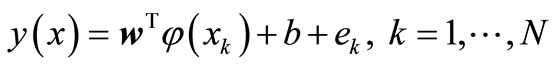 . (2)
. (2)
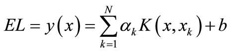
where ek = error variable and γ = regularization parameter. The following equation for EL prediction has been obtained by solving the above optimization problem [18-19].
 (3)
(3)
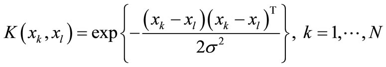
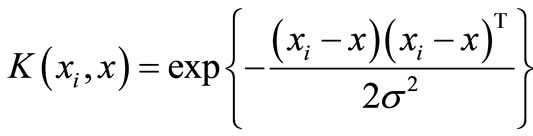
where K(x, xk) is kernel function. The radial basis function has been used as kernel function in this analysis. The radial basis function is given by
 (4)
(4)
where σ is the width of radial basis function.
The above LSSVM has been adopted for determination of EL. The data are collected from a reservoir in Anand Sagar, Shegaon (India). The data of evaporation loss were collected for one year only. Whereas, the other data for a period of fifteen year (from 1990 to 2004) were obtained from a full climatic station at Manasgaon, about 9 Km from Shegaon, lying under water resources division, Amravati Hydrology Project (Maharashtra, India). The dataset contains information about 48 cases. The data have been divided into two sub-sets; a training dataset, to construct the model, and a testing dataset to estimate the model performance. So, for our study a set of 34 data are considered as the training dataset and remaining set of 14 data are considered as the testing dataset. The data are scaled between 0 and 1. This study uses radial basis function
 , where σ is the width of the radial basis function) as a kernel function. The design values of the γ and σ will be determined during the training of LSSVM.
In this study, a sensitivity analysis has been done to extract the cause and effect relationship between the inputs and outputs of the LSSVM model. The basic idea is that each input of the model is offset slightly and the corresponding change in the output is reported. The procedure has been taken from the work of [20]. According to [20], the sensitivity (S) of each input parameter has been calculated by the following formula
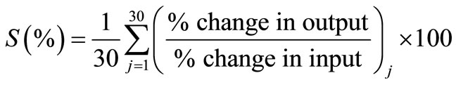 (5)
(5)
The analysis has been carried out on the trained LSSVM model by varying each of input parameter, one at a time, at a constant rate of 20%. In the present study, training, testing and sensitivity analysis of LSSVM have been carried out by using MATLAB.
3. Results and Discussion
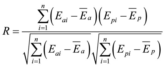
Different combinations of γ and σ have been tried to get the best result. The design values of γ and σ are 100 and 2 respectively. The performance of training dataset has been computed by using the design values of γ and σ. The value of Coefficient of Correlation(R) for training has been determined by using the following equation.
 (6)
(6)
where Eai and Epi are the actual and predicted E values, respectively,  and
and  are mean of actual and predicted E values corresponding to n patterns. For good model, the value of R should be close to one. Figure 1 illustrates the performance of training dataset. For training dataset, the value of R is 0.998. Therefore, the developed LSSVM has captured the input and output relationship very well. Now, the performance of the developed LSSVM has been examined for the testing dataset. Figure 2 depicts the performance of testing dataset. It is observed from figure 2 that the value of R is 0.996 for testing dataset. So, the developed LSSVM model can be used as a practical tool for determination of EL. The developed LSSVM model also gives the following equation
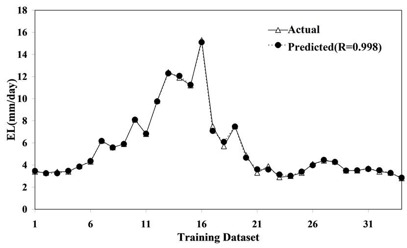
Figure 1. Performance of training dataset.
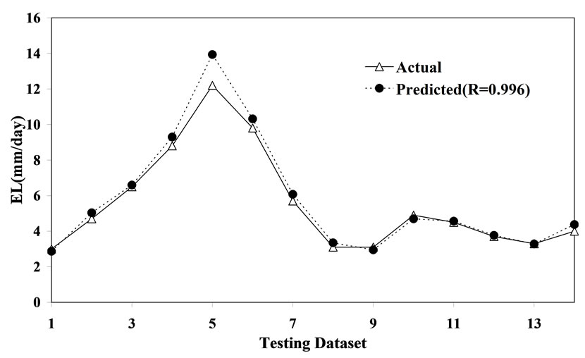
Figure 2. Performance testing dataset.
{by putting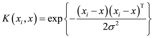 , σ = 2 and b = 0.3413 in “(4)”} for prediction of EL.
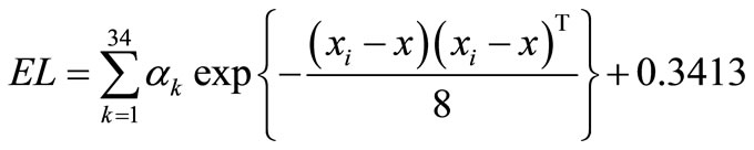 (7)
(7)
The values of α have been given in figure 3.
Error bar has been also computed by using the developed LSSVM model. Figures 4 and 5 depict the error bar of training and testing dataset respectively. The predicted error bar can be used to determine confidence interval. The results of sensitivity analysis have been shown in figure 6. It is observed from figure 6 that T has maximum effect of EL followed by RH, SH, and WS.
A comparative study has been done between the developed LSSVM and ANN model developed by “Deswal and Pal (2008)”. The obtained R and Root Mean Square Error (RMSE) value from ANN model is 0.960 and 0.865. The developed LSSVM model predicts EL value with an accuracy of R = 0.996 and RMSE = 0.539. Therefore, the performance of the developed LSSVM model is slightly better than ANN model. ANN model uses many parameters such as the number of hidden lay-
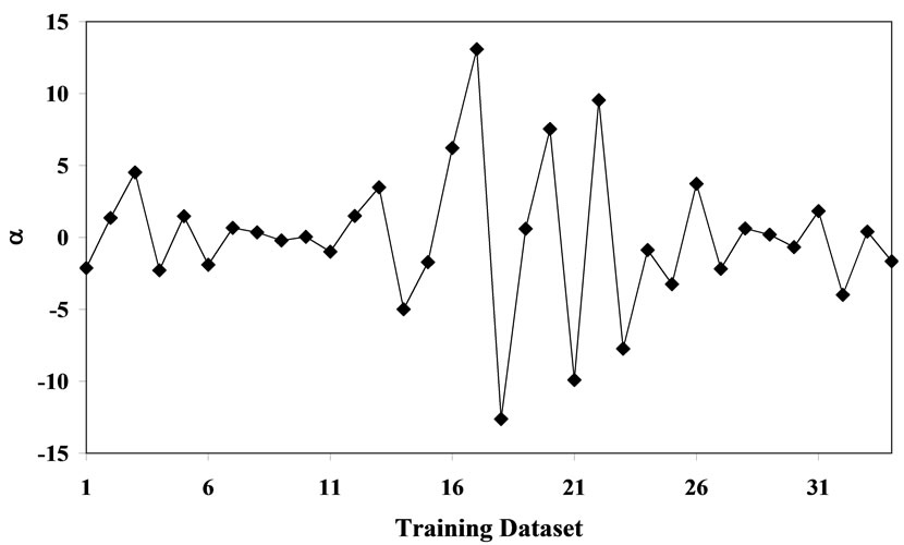
Figure 3. values of α.
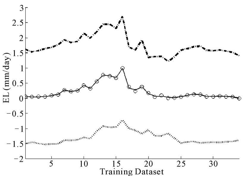
Figure 4. 95% error bar for training dataset.
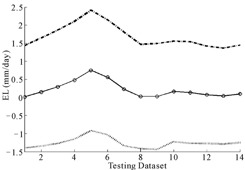
Figure 5. 95% error bar for testing dataset.
ers, number of hidden nodes, learning rate, momentum term, number of training epochs, transfer functions, and weight initialization methods. Whereas, LSSVM model uses two parameters γ and σ.
4. Conclusions
This study has described LSSVM model for prediction of
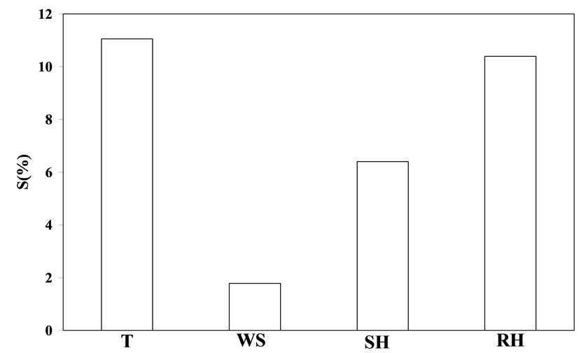
Figure 6. Sensitivity analysis of input parameters.
EL in reservoirs. 48 datasets have been utilized to develop LSSVM model. The performance of LSSVM model is encouraging. User can use the developed equation for prediction of EL. The developed LSSVM also gives prediction uncertainty. Sensitivity analysis indicates that T has maximum effect on EL. This article shows that the developed LSSVM is a robust model for prediction of EL.
5. REFERENCES
- E. D. Eaton, “Control of Evaporation Losses,” United States Government Printing Office, Washington, 1958.
- V. P. Singh and C.Y. Xu, “Evaluation and Generalization of 13 Mass Transfer Equations for Determining Free Water Evaporation,” Hydrological Processes, Vol. 11, 1997, pp. 311-323. doi:10.1002/(SICI)1099-1085(19970315)11:3<311::AID-HYP446>3.0.CO;2-Y
- R. B. Stewart and W. R. Rouse, “A Simple Method for Determining the Evaporation from Shallow Lakes and Ponds,” Water Resources Research, Vol. 12, 1976, pp. 623- 627. doi:10.1029/WR012i004p00623
- H. A. R. D. Bruin, “A Simple Model for Shallow Lake Evaporation,” Journal of Applied Meteorology, Vol. 17, 1978, pp. 1132-1134. doi:10.1175/1520-0450(1978)017<1132:ASMFSL>2.0.CO;2
- M. E. Anderson and H. E. Jobson, “Comparison of Techniques for Estimating Annual Lake Evaporation Using Climatological Data,” Water Resources Research, Vol. 18, 1982, pp. 630-636. doi:10.1029/WR018i003p00630
- W. Abtew, “Evaporation Estimation for Lake Okeechobee in South Florida,” Journal of Irrigation and Drainage Engineering, Vol. 127, 2001, pp. 140-147. doi:10.1061/(ASCE)0733-9437(2001)127:3(140)
- S. Murthy and S. Gawande, “Effect of Metrological Parameters on Evaporation in Small Reservoirs ‘Anand Sagar’ Shegaon - A Case Study,” Journal of Prudushan Nirmulan, Vol. 3, No. 2, 2006, pp. 52-56.
- S. Deswal and P. Mahesh, “Artificial Neural Network Based Modeling of Evaporation Losses in Reservoirs,” International Journal of Mathematical, Physical and Engineering Sciences, Vol. 2, No. 4, 2008, pp.177-181.
- D. Park and L. R. Rilett, “Forecasting Freeway Link Travel Times with a Multi-Layer Feed forward Neural Network,” Computer Aided Civil and Infrastructure Engineering, Vol. 14, 1999, pp. 358-367. doi:10.1111/0885-9507.00154
- V. Kecman, “Learning and Soft Computing: Support Vector Machines, Neural Networks, and Fuzzy Logic Models,” The MIT press, Cambridge, 2001.
- J. A. K. Suykens, L. Lukas, D. P. Van, M. B. De and J. Vandewalle, “Least Squares Support Vector Machine Classifiers: A Large Scale Algorithm,” Proceedings of European Conference on Circuit Theory and Design, Stresa, 1999, pp. 839-842.
- A. J. Smola, “Learning with Kernels,” Ph.D. dissertation, GMD, Birlinghoven, Germany, 1998.
- X. D. Wang and M. Y. Ye, “Nonlinear Dynamic System Identification Using Least Squares Support Vector Machine Regression,” Proceedings of the Third International Conference on Machine Learning and Cybernetics, Shanghai, 2004, pp. 26-29.
- P. Samui and T. G. Sitharam, “Least-Square Support Vector Machine Applied to Settlement of Shallow Foundations on Cohesionless Soils,” International Journal of Numerical and Analytical Method in Geomechanics, Vol. 32, No.17, 2008, pp. 2033-2043. doi:10.1002/nag.731
- A. Baylara, D. Hanbay and M. Batan, “Application of Least Square Support Vector Machines in the Prediction of Aeration Performance of Plunging Overfall Jets from Weirs”, Expert Systems with Applications, Vol. 36, No.4, 2009, pp. 8368-8374. doi:10.1016/j.eswa.2008.10.061
- V. Vapnik and A. Lerner, “Pattern Recognition Using Generalizd Portait Method,” Automation and Remote Control, Vol. 24, 1963, pp. 774-780.
- J. A. K. Suykens, B. J. De, L. Lukas and J. Vandewalle, “Weighted Least Squares Support Vector Machines: Robustness and Sparse Approximation”, Neurocomputing, Vol. 48, No. 1-4, 2002, pp. 85-105. doi:10.1016/S0925-2312(01)00644-0
- A. Smola and B. Scholkopf, “On a Kernel Based Method for Pattern Recognition, Regression, Approximation and Operator Inversion,” Algorithmica, Vol. 22, 1998, pp. 211-231. doi:10.1007/PL00013831
- V. N. Vapnik, “Statistical Learning Theory,” Wiley, New York, 1998.
- S. Y. Liong, W. H. Lim and G. N. Paudyal, “River Stage Forecasting in Bangladesh: Neural Network Approach,” Journal of Computing in Civil Engineering, Vol. 14, No.1, 2000, pp.1-8.doi:10.1061/(ASCE)0887-3801(2000)14:1(1)