Journal of Modern Physics
Vol.5 No.8(2014), Article ID:46473,13 pages DOI:10.4236/jmp.2014.58081
Bose-Einstein Condensation of Confined Magnons in Nanostructures
Lawrence H. Bennett, Edward Della Torre
The George Washington University, Washington DC, USA
Email: edt@gwu.edu
Copyright © 2014 by authors and Scientific Research Publishing Inc.
This work is licensed under the Creative Commons Attribution International License (CC BY).
http://creativecommons.org/licenses/by/4.0/


Received 12 December 2013; revised 13 January 2014; accepted 11 February 2014
ABSTRACT
A number of diverse kinds of magnetic experiments are shown to lead to the observation of a Bose-Einstein condensation of magnons in some nanostructures, especially in Fe and in Co/Pt. The experiments include 1) the measurement of magnetic aftereffect, 2) measurements of Néel’s fluctuation field, including an estimate of activation volume, 3) the measurement of the energy gap which provides a lower limit on the BEC temperature, 4) using Lagrange multipliers in the quantum thermodynamics of magnons, and 5) the observation of a visible anomaly in the Bloch T3/2 law for the temperature dependence of magnetization of nanostructured ferromagnets.
Keywords:Bose-Einstein Statistics, Aftereffect, Bloch T3/2 Law, Chemical Potential, Arrhenius Law

1. Introduction
The occupation of a single quantum state by a large fraction of bosons at low temperatures [1] was predicted by Bose and Einstein in the 1920s. The quest for Bose-Einstein condensation (BEC) in a dilute atomic gas was achieved [2] in 1995 using laser-cooling to reach ultra-cold temperatures of 20 nK. BEC of dilute atomic gases, now regularly created in a number of laboratories around the world, have led to a wide range of unanticipated applications. Especially exciting is the effort to use BEC for the manipulation of quantum information, entanglement, and topological order.
The study of atomic BEC has yielded rich dividends. A promising extension is to magnons—spin-wave quanta that behave as bosonic quasiparticles—in magnetic nanoparticles. This system has unique characteristics differentiating it from atomic BEC, creating the potential for a whole new variety of interesting behaviors and applications that include high-temperature Bose-Einstein condensation and novel nanomagnetic devices. BoseEinstein condensation in atoms [2] and photons [3] is now an accepted phenomenon. Recent research [4] -[10] focuses on gaining understanding in different quasi-particles, including photons, phonons, gluons, and magnons.
Magnons are quantized spin waves created when the magnetic moments of an electron spin change due to variation in magnetic field across a crystal lattice. The annihilation and the creation of magnons thus occur when the electron undergoes a spin-flip. The magnetization of the material also depends upon the magnon density [11] , which increases or decreases with temperature. The magnon density is also affected by the electron-magnon scattering in the unoccupied region of the transition metals [12] . To undergo BEC, it is necessary to either increase the density of bosons or lower the temperature. The consensus on whether these magnons obey BoseEinstein statistics is still to be reached. Numerous claims were made to prove it [4] [6] [13] [14] but still the true nature of it is yet to be understood. In a quasi-equilibrium state, quasiparticles such as magnons show BEC [15] experimentally.
The BEC of quasi-equilibrium magnons has been achieved at room temperature by exciting more magnons into a gas of quasi-equilibrium magnons with a non-zero chemical potential through microwave pumping. However, some physicists [16] [17] are hesitant to accept the phenomenon observed by Demokritov et al. [6] , as BEC and are more willing to perceive it as coherent quantum state or BEC like behavior. Zvyagin [18] observes that “Despite the question of whether Bose-Einstein condensation is the right term to apply to the observed phenomena, coherent quantum states of magnons, either near phase transitions [4] [9] [18] [19] , or induced by the paramagnetic pumping [6] , are among the most interesting phenomena of modern condensed matter physics”.
Magnons and their strong confinement [6] induce gaps in their energy spectra. The lowest lying of the gaps provides a first approximation to the temperature of BEC formation. However, BEC formation is also influenced by the density of the magnons. This modifies the energy gap, which can cause the significant changes in the predicted BEC temperature. The behavior and the magnetic properties of the magnonic crystals vary significantly with the magnon density and temperature [13] . For the material to behave as BEC, it must be cooled into its lowest possible energy state. However, if the temperature is increased beyond the gap temperature (the temperature that moves the material from lowest energy state to the next) [20] [21] , the behavior changes and it is considered as lower limit on attaining BEC. For a particular nanometer size length of material, the material is in its ferromagnetic state above its gap temperature and is a Bose-Einstein condensate below it. By creating higher magnon density [22] , the Bose-Einstein temperature and associated phenomenon could occur at even higher temperatures.
In nanoparticles, finite size and surface effects, anisotropy and influence of geometry, all have significant impact on magnon characteristics, including lifetimes and scattering processes. At nanometers length [6] [23] with different lattice types and particle shapes, the blocking temperature becomes important. If the temperature is increased beyond the gap temperature (the temperature that moves the material from lowest energy state to the next) [24] [25] , the behavior changes and it is a lower limit on attaining BEC. For a particular nanometer size length of material, the material is in its ferromagnetic state above its gap temperature and is Bose-Einstein condensate below it. The rough shape of a phase diagram describing the critical behavior of magnons in magnetic nanoparticles, delineating the 1) Bose-Einstein condensate, 2) a superparamagnetic, and 3) ferromagnetic phases in nanostructures has been pictured [26] and shown in Figure 1.
In nanoparticles, finite size and surface effects, anisotropy, and influence of geometry have significant impact on magnon characteristics, including lifetimes and scattering processes. Also, at nanometers length [23] [27] [28] with different lattice types and particle shapes. The material is a Bose-Einstein condensate below the blocking temperature and is in a superparamagnetic state above that.
In a study of magnetic aftereffect we observed non-Arrhenius behavior, in that the decay rates did not increase monotonically with temperature as expected, but instead had a low temperature peak. We analyzed the behavior of the fluctuation fields and again found non-Arrhenius behavior. We attributed the peak to a possible BoseEinstein condensation. We therefore computed the energy gap in a confined space in order to determine the condensation temperature. Since magnons are bosons, we assumed that they obeyed Bose-Einstein statistics and found that the observed behavior could be explained by a linear variation of the chemical potential with temperature. The temperature intercept of this variation was a positive absolute temperature. Below that temperature the chemical potential is zero. A nonzero chemical potential is possible in quasi-equilibrium, where the number is approximately constant. The slope of the linear portion above TB according to Maxwell’s equations is equal to the entropy of the system. The entropy was the same in all the aftereffect experiments, since the samples were all initially DC demagnetized. A further test of this analysis was to measure Bloch’s T3l2 law where we found an

Figure 1. Approximate shape of a phase diagram delineating the boundaries of the regions.
anomaly. We again explained this anomaly by Bose-Einstein condensation and got good agreement with experiment.
2. Method
2.1. Non-Arrhenius Behavior in Magnetic Aftereffect
When a ferromagnetic material is magnetized, a reversed field can more or less demagnetize it. Maintaining the field and temperature constant, the magnetization then decays slowly (magnetic aftereffect) towards the anhysteretic ground state. It is expected, and it is found in many magnetic materials, that the decay of magnetization, measured by thermal magnetic aftereffect experiments, becomes smaller when the temperature is cooled. This Arrhenius behavior is a consequence of Maxwell-Boltzmann statistics. In some nanostructured ferromagnets, a peculiar temperature dependence of the thermal magnetic aftereffect has been reported [29] , namely an increase in decay rate as the temperature is lowered from room temperature, peaking at some low temperature. This nonArrhenius behavior could be explained by assuming that the magnons responsible for the decay obeyed BoseEinstein (BE) statistics with a non-zero chemical potential, and that the peak is connected with the Bose-Einstein condensation temperature, TB. In a classic paper on magnetic aftereffect [30] , the Preisach-Arrhenius (PA) model is an approach built on fundamental thermodynamic principles and predicts the decay rate at any holding field very accurately. The PA model uses the Arrhenius-Néel law [31] to determine the aftereffect.
2.2. Decay Rates
Magnetic aftereffect, the slow decay of the magnetization toward the anhysteretic state, is a non-equilibrium process that is controlled by 1) overcoming a distribution of energy barriers by thermal activation, and by 2) the chemical potential, ζ, that determines how many thermal quanta are available. The former is predominant in the remanence state and the latter in the demagnetized state. Arrhenius behavior implies a monotonic increase in the decay rate with increasing temperature. Normally, this is just what is seen in most materials. However, when the magnon energy distribution, which obeys quantum statistics, has a finite Bose-Einstein condensation at a BEC temperature, TB, a peak is observed in the maximum decay rate vs. temperature at TB. Such a peak has been observed in some nano-magnetic materials. For example, decay rate studies of the temperature dependence of the magnetic aftereffect of Fe nano-particles [32] shows a large peak at ∼30 K, as seen in Figure 2 for nano-particle powder. Assuming [33] that the magnons responsible for the decay obeyed Bose-Einstein (BE) statistics with a linear temperature-dependent chemical potential, ζ, obeying [34]
 (1)
(1)
where H, M, S, v, p, and T are the magnetic field, the magnetization, the entropy, the volume, the pressure, and the temperature, respectively. Thus, under constant pressure and magnetization

Figure 2. Maximum decay rate, R, vs. temperature for an Fe nano-particle powder, showing a peak at ∼30 K. The solid line is a fit to the theory.
 (2)
(2)
Unless S ≡ 0, ζ cannot be zero for all temperatures, and it is well known that the entropy is not zero, at least in the demagnetized state. For any given magnetic state, the entropy, S, is a constant. Assuming a chemical potential variation from Equation (2) with two adjustable parameters, S and TB, for the Fe nanoparticles yields Figure 3, which shows the chemical potential needed to provide the fit shown in Figure 2. Similar behavior in metal particle recording tape is shown in Figure 4 and the corresponding chemical potential is shown in Figure 7.
To understand fully this non-Arrhenius behavior, it is useful to elaborate their thermodynamic framework. For simplicity, assume that the basic particles are all identical and perfectly ordered. If the aftereffect is measured at each temperature, by starting from the same magnetic state, then the distribution will have the same entropy, and thus the same chemical potential. Hence, the slope of the chemical potential with temperature should be constant, as found experimentally.
Similar results were found in nano-particulate (metal-particle tape) media [35] . In this case, as in the nanoparticles, we found that the maximum decay rate, R, had a low-temperature peak in contrast to the expected monotonic Arrhenius behavior, as seen in Figure 4. Again, except at the lowest temperatures, the chemical potential is linear with temperature (Figure 7). Note that [36] , in neither the nanograin iron, nor the nano-particulate media, is there any other explanation for the peak, i.e., there are no phase changes, no changes in the easy direction of magnetization, no movement of interstitial atoms, or other significant crystallographic or magnetic changes.
The magnetic aftereffect can be modeled as due to interactions between magnons (spin waves) and hysterons (magnetic entities acting as a single magnetic moment). If the energy of the magnon is less than that of the barrier energy for a reversal of the magnetization, then the collision is purely elastic. On the other hand, if the magnon has greater energy than the barrier energy, then there is a finite probability that the hysteron will reverse. The frequency of particle reversal, f, due to magnons is the product of the attempt frequency fA and the probability that the magnon has sufficient energy to overcome the energy barrier to reversal, p(E > EB). If the energy distribution obeys Maxwell-Boltzmann (MB) statistics and the density of states in energy space is uniform, then the rate equation is given by the Arrhenius law. On the contrary, if the energy distribution obeys quantum statistics or the density of states in energy space is not uniform, non-Arrhenius behavior would be observed. In general, the number of particles that in a given collision have energy greater than EB is obtained by integrating over all possible energies, that is
 (3)
(3)
where n(E) is the expectation value of the number of particles in a state that has energy E, and δ(E) is the density of states in energy space.

Figure 3. Chemical potential required to obtain the fit of R shown in Figure 2. The curvature near ζ = 0 is attributed to size dispersion.
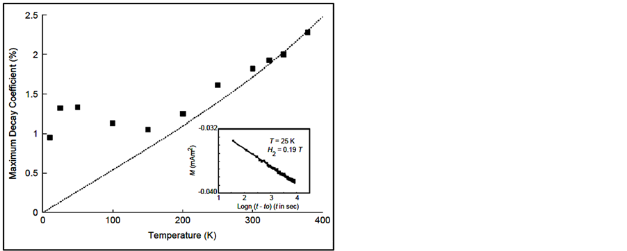
Figure 4. The maximum decay coefficient as a function of temperature for the particulate iron in a recording tape media. The dotted line is a plot of the decay assuming classical statistics and using measured values of the parameters. The inset shows a typical measurement (M vs. T) of the decay coefficient.
2.3. Fluctuation Fields
A different type of decay was observed in measurements from 4 K to room temperature [31] on a film that was nominally a nanostructured (3 nm Co/2 nm Pt) [15] magnetic multilayer film grown on a sapphire substrate at 573 K. Analysis of this film showed that it actually had a nanopillar structure [37] of about 30 nm height and a similar diameter. The magnetization is perpendicular to the film and arises from these aligned nano-pillars. The magnetization decay rate in the cobalt-platinum is much faster than those of the aforementioned nano-particulate systems. In this case, it is possible to view the entire sigmoidal shaped decay curve. Such decay curves, in log time, are shown in Figure 5 for various fields near the coercivity. This permits an alternate method of analysis: characterizing the aftereffect in terms of the fluctuation field introduced by Néel [33] .
This experiment provides an especially robust observation of the BE condensation of the magnons. The fluctuation field, Hf, as expanded by Street and Brown [38] , can be viewed as the driving force in a magnetic aftereffect. It is normally given by
 (4)
(4)
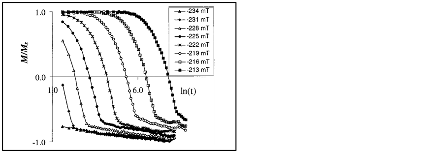
Figure 5. Measured aftereffect curves in a (3 Co/10 Pt)15 multilayer film.
where V is the activation volume of the individual magnetic entity (“particle”) and Ms is the saturation magnetization. Many investigators incorporate the chemical potential term into the attempt frequency, hence they find the activation volume is a significant function of temperature, which is contrary to having a given physical volume [39] .
The technique to obtain the fluctuation field from the decay curves involves scaling and translating them. If there is a negligible reversible magnetization and negligible inter-particle interactions, then it can be shown [40] that all the aftereffect curves and the major loop are similar in a geometric sense. The similarity of the major loop with the aftereffect curve is a direct method of confirming the Wohlfarth hypothesis since the field that maximizes the slope of the major loop, which is the susceptibility, also maximizes the slope of the aftereffect decay.
Since this Co/Pt satisfied the criteria in the previous paragraph, a new technique was developed [41] to measure the fluctuation field that consisted of finding two parameters: a horizontal translation and a scaling to account for the difference in anhysteretic magnetization at different holding fields.
The technique is performed by mapping each of the curves onto the major hysteresis loop, in order to normalize them so that they all extend from positive saturation to negative saturation. Since the horizontal translation is directly proportional to the ratio of the holding field to the fluctuation field, it is possible to determine the fluctuation field from the slope of the translation versus the holding field, as obtained from a linear regression of the data in Figure 6.
The fluctuation field at each temperature is obtained from the slope of the required translation as a function of the holding field. As seen in Figure 7, the relaxation does not slow down as the temperature is lowered but, instead increases and reaches a peak at 14 K, which we identify as a Bose-Einstein condensation temperature, TB. The fluctuation field is theoretically (under some simplifying assumptions) directly proportional to the absolute temperature below the BE condensation temperature, TB, of the magnons (see Figure 9). Below TB the fluctuation field mimics the Arrhenius law. The field has a sharp peak at the TB, then decreases until it approaches a constant value asymptotically from below for higher temperatures. The chemical potential, ζ, obtained from the fit shown in Figure 8 using the data in Figure 9.
Note that ζ = 0 below TB (which is a requirement for having a BEC), and linear above. As already noted, these peaks in the magnetic aftereffect present particularly robust indications of a Bose-Einstein phase transition.
For a given material, there is a critical condensation temperature below which there is no peak in the fluctuation field. This is illustrated in Figure 10, where this temperature is 10 K. When the condensation temperature is above this value, the fluctuation field increases linearly, i.e., following the Arrhenius law, until that temperature and above it, the fluctuation field decreases as the temperature continues to increase. This calculation assumes that the energy barrier is temperature independent. For a temperature-dependent energy barrier, the curve will eventually be monotonically increasing.
2.4. Energy Gap in a Confined Space
There have been several discussions related [42] -[44] to the energy gap in a finite size material. The gap tem-
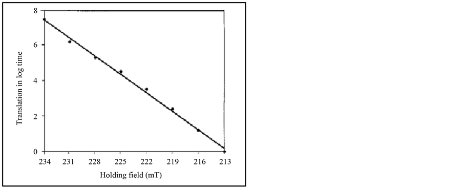
Figure 6. The translation, in log time, versus the holding field, in mT, from the CoPt nanopillar data of Figure 5. The solid line is a linear regression of the data.
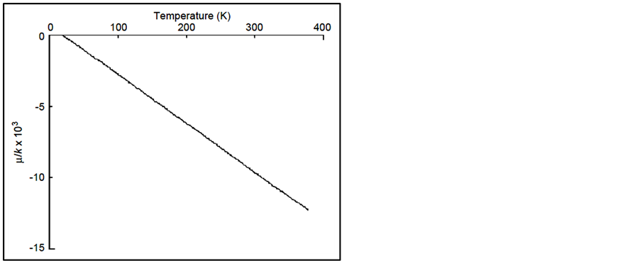
Figure 7. Variation of ζ/k, in units of 103 K, for the recording tape.
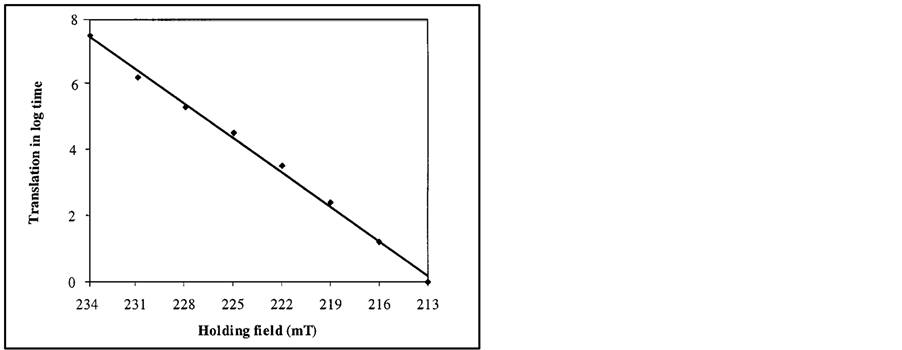
Figure 8. The translation in log time, versus the holding field, in mT, from the Co/Pt nanopillar data of Figure 6. The solid line is a linear regression of the data.

Figure 9. Temperature variation of the fluctuation field, Hf, in a Co/Pt nanostructure.

Figure 10. The effect of TBE on the fluctuation field, when Hf and EB are constant.
perature, Tgap, is the lower bound for the BEC temperature. This means that in Figure 3, the line separating the BEC from the ferromagnetic region can be substantially higher.
The energy Ei of a magnon in state i, for a simple body-centered or face centered cubic lattice, is given by [45]
 (5)
(5)
where J is the exchange constant, ki is the wave vector associated with state i, and a is the lattice spacing, that is, the distance between corner atoms in the unit cell. The wave vector can be expressed in terms of the de Broglie wavelength, λi, as
 (6)
(6)
The smallest non-zero wave vector is obtained by setting λi equal to the largest dimension of the particle. The BEC temperature is estimated by computing the gap temperature, Tgap. This temperature is a lower bound on TB, which could be appreciably larger. It is obtained by setting the lowest non-zero magnon energy equal to the thermal energy. Using the equipartition of energy, this energy is 1/2kBT, where kB is Boltzmann’s constant and T is the temperature in K, the thermal de Broglie wavelength for a magnon in a spherical particle
 (7)
(7)
and the gap temperature, Tgap, is found by setting λ equal to the particle’s diameter, d, and solving for T we obtain Tgap, which is a lower bound TB. Thus,
 (8)
(8)
For iron, using the lattice constant a of 0.4 nm, and the accepted [46] J value of 2.16 × 10‒21 J, this would become 12,270 (a/d)2. These parameters, J and a, are approximately characteristic of the iron and cobalt nanostructures.
2.5. Quantum Thermodynamics of Magnons
Magnons are quasi-particles that interact with the spin of electrons to change the magnetization of the material. In order to conserve angular momentum, since the electrons have spin , the difference between two electron states must be an integer. Therefore, magnons are bosons. When the magnons are in equilibrium, they obey Bose-Einstein statistics with zero chemical potential, but when they are in quasi-equilibrium, but not in true equilibrium. That is when the number of magnons is essentially constant, they obey Bose-Einstein statistics with nonzero chemical potential, ζ. The number of magnons can be kept essentially constant if new magnons are created at the same rate at which they are destroyed. This can be described by noting that the magnons are in quasi-equilibrium.
The chemical potential has to be adjusted so that the sum of (1) over all states is equal to the total number of particles. In order to find the quasi-equilibrium state, we have to find the state with the maximum thermodynamic probability, that i the entropy, subject to the constraints that the total energy and the number of particles is constant. This is generally solved using Lagrange multipliers so that the problem can be solved as an unconstrained maximization. The Lagrange multiplier that keeps the number of magnons constant is the chemical potential.
Thus, the number of magnons with energy Ei, is given by
 (9)
(9)
Then the chemical potential is chosen by letting
 (10)
(10)
where N is the total number of particles. Under quasi-equilibrium, ζ is negative and its magnitude grows larger with increasing temperature. In that case, since Ei is positive, as the temperature increases, the statistics approach classical statistics as in the correspondence principle, since the exponential term is so large that the −1 can be neglected. Another way of looking at it is, if the exponential term in the denominator is very large, the magnon wavelength is small and so there is negligible overlap of the wave functions, and it is possible to distinguish the particles without violating the exclusion principle.
Since the chemical potential is a negative number, it has the effect of reducing the number of magnons in all energy states. This is necessary in order to explain the extremely slow decay of aftereffect at room temperature in the presence of an attempt frequency of the order of 109.
Kittel has shown [47] -[50] that the number of magnons at any temperature is directly proportional to the difference between the saturation magnetization occurring at that temperature to that at 0 K. For ferromagnetic materials such as iron, this is only a few percent of the saturation magnetization at room temperature. Furthermore, since the change in magnetization with time in these materials is extremely slow, the number of magnons is essentially a constant. While TB can be made larger by increasing the magnon density, this review only examines the theoretical dependence of TB on the nanoparticle size, which is easily accessible experimentally.
Magnons (spin-wave quanta) behave like a gas of weakly interacting particles obeying Bose-Einstein statistics. When confined in a small nanoparticle (e.g., an iron sphere with diameter on the order of 1 - 10 nm), the allowed magnon wave vectors ki are quantized, giving a discrete spectrum Ei with an energy gap, Egap = E1 − E0, between the lowest and next to lowest allowed states. If the magnons are in equilibrium at temperature T, then the number in a state i, is given by the Bose-Einstein distribution function.
2.6. Quasi-Equilibrium―Number of Magnons
In measurements of thermal magnetic aftereffect, the magnetization decay may be so small, that for some measurements the decay is only a small fraction of a per cent. Thus, when measuring the magnetization as a function of temperature, at any given temperature, the magnetization is essentially constant. Such a system is said to be in quasi-equilibrium. Since the fractional change in magnetization is equal to the number of magnons divided by the number of electrons, the number of magnons in these cases is also constant. Thus, when measuring the saturation magnetization as a function of temperature, as in the case of the Co/Pt nanostructure, the magnetization is not a measurable function of time and thus, the number of magnons is constant. In the case of the decay measurements, if the observation window is short enough, the magnetization changes almost imperceptibly, and again the number of magnons is constant. When maximizing the thermodynamic probability, the method of Lagrange multipliers is used to permit only variations, if the number of particles is constant, and ζ is that multiplier.
In an open system, or in one that bosons can be created or destroyed, the chemical potential must be zero. However, if the system is far from equilibrium, but is changing sufficiently slowly so that it reaches a quasiequilibrium, a non-zero chemical potential is permitted. Can quasiparticles, such as magnons, whose numbers are not conserved but have finite lifetimes undergo Bose-Einstein condensation? The consensus on this issue [16] , reached about a decade ago, is that if the lifetime of the particles is much longer than the time they need to scatter with each other, condensation is possible. It is thus appropriate to say that if the observations do not include all possible tests, the system is either BEC or BEC-like.
2.7. Anomaly in the Bloch T3/2 Law in Nanostructures
Bloch’s [48] T3/2 law of variation of saturation moment with temperature [7] is regarded as the fundamental law of ferromagnetism. The decrease of the saturation moment with increasing temperature in a bulk ferromagnetic material is determined by the “stiffness” of the exchange coupling which tends to align the spins of all the atoms parallel [8] . The law has been tested in a careful set of experiments [9] in single crystals of ferromagnetic metals.
The law assumed that the chemical potential was zero. A correction to the chemical potential variation, characteristic of BE condensation, suggested above showed that the magnetization obeyed the Bloch’s T3l2 law up to the condensation temperature, but above that temperature it is asymptotic to another T3l2 law, with different coefficients.
The fractional decrease in saturation magnetization, M, is
 (11)
(11)
which is the same as the traditionally derived case discussed by Kittel [47] . If S = 0 then, ζ = 0, as in perfect single crystals, this becomes
 (12)
(12)
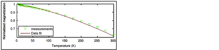
Measurements in nanostructures [4] showed that this correction, illustrated in Figure 11, is accurate virtually to room temperature, further demonstrating that these confined magnons form a Bose-Einstein condensate.
3. Results
Bose-Einstein condensation of magnons confined in nanostructures has been established by a variety of different
 (a)
(a)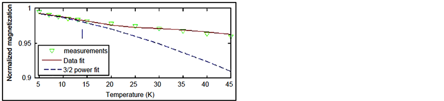 (b)
(b)
Figure 11. Saturation magnetization vs. temperature for the Co/ Pt nanopillars.
experiments all giving the same results for a particular specimen. These results are obtained in quasi-equilibrium. For a typical magnon, magnon-phonon processes are slower than magnon-magnon processes. This means that spin-spin equilibrium is established more rapidly than spin-lattice equilibrium [52] .
Of special note is the identification of the peak seen in thermal magnetic aftereffect versus temperature. As the temperature is lowered, “The elegant and wide-ranging Arrhenius equation tells us how much slower” [53] Atzmony, et al. [12] , noticed the peaks and said that they were non-Arrhenius, but had no explanation. A number of other reports of similar peaks were never explained or even commented on. The Arrhenius equation is based on classical thermodynamics. Since the magnons are bosons, Bose-Einstein thermodynamics provides excellent agreement between experiment and theory [4] [11] [15] [29] [30] [32] [33] [35] -[37] [39] -[41] .
4. Discussion
The study of atomic BEC has yielded rich dividends. A promising extension is to magnons—spin-wave quanta that behave as bosonic quasiparticles—in magnetic nanoparticles. This system has unique characteristics differrentiating it from atomic BEC, creating the potential for a whole new variety of interesting behaviors and applications that include novel nanomagnetic devices.
Further work is needed to determine the relationship between nanostructural morphology (size, shape, etc.) and the Bose-Einstein condensation temperature.
A most important point is that a magnon propagates spatially all over the magnet. By this propagation, quantum coherence is established between spatially separated points. Therefore, by exciting a macroscopic number of magnons, one can easily construct states with huge entanglement [54] . Entanglement is a basis for quantum computation.
The BEC has important significance to magnetic resonance: Below TB, the entropy is zero, and is essentially constant above that. If the Gilbert damping is related to the entropy, then very narrow line widths are possible below TB. This has implications for low loss or sharp filters for microwave devices.
A condensate is a quantum system. It follows, therefore, that its properties depend in large part on the measurements you can perform on it. Condensates are open systems; some dynamical processes cause members of the condensate to be lost while other processes add particles to it. This does not imply a zero chemical potential, e.g., introductory chemistry students routinely calculate the chemical potential for the reaction:  [55] . Since BE condensates are not made in pure states, at the most fundamental level, there should be a highly entangled state of the particles forming the condensate plus the environment.
5. Conclusion
Bose-Einstein (or Bose-Einstein-like) condensation in metallic nanostructures has been observed using a variety of magnetic signatures [4] [11] [15] [26] [29] [30] [32] [33] [35] -[37] [39] -[41] . All of the methods gave comparable results. Especially illuminating was the measured graph of chemical potential versus temperature, which in some alloys was exactly as statistical mechanics text books described the ideal case of BEC, i.e., zero chemical potential up to the BEC transition point, and then negative and linear above that temperature.
Acknowledgements
The work is partially supported by National Science Foundation under Contract no. 0733526 and no. 1031619. We would also like to thank Hatem ElBidweihy, Chidubem Nwokoye and Ali Jamali for their help in preparing the manuscript.
References
- Bose, S. (1924) Zeitschrift für Physik, 26, 178-181. Einstein, A. and Sitzungsber, K. (1925) Preuss. Akad. Wiss., Phys. Math. Kl. 3. http://dx.doi.org/10.1007/BF01327326
- Cornell, E.A., Ketterle, W. and Wieman, C.E. http://nobelprize.org/nobelprizes/physics/laureates/2001/
- Anglin, J. (2010) Nature, 468, 517-518. http://dx.doi.org/10.1038/468517a
- Della Torre, E., Bennett, L.H. and Watson, R.E. (2005) Physical Review Letters, 94, Article ID: 147210. http://dx.doi.org/10.1103/PhysRevLett.94.147210
- Kasprzak, J., Richard, M., Kundermann, S., Baas, A., Jeambrun, P., Keeling, J.M.J., Marchetti, F.M., Szymańska, M.H., André, R., Staehli, J.L., Savona, V., Littlewood, P.B., Deveaud, B. and Dang, L.S. (2006) Nature, 443, 409-414. http://dx.doi.org/10.1038/nature05131
- Demokritov, S.O., Demidov, V.E., Dzyapko, O., Melkov, G.A., Serga, A.A., Hillebrands, B. and Slavin, A.N. (2006) Nature, 443, 430-433. http://dx.doi.org/10.1038/nature05117
- Eisenstein, J.P. and MacDonald, A.H. (2004) Nature, 432, 691-694. http://dx.doi.org/10.1038/nature03081
- Coldea, R., Tennant, D.A., Habicht, K., Smeibidl, P., Walters, C. and Tylczynski, Z. (2002) Physical Review Letters, 88, Article ID: 137203. http://dx.doi.org/10.1103/PhysRevLett.88.137203
- Radu, T., Wilhelm, H., Yushankhai, V., Kovrizhin, D., Coldea, R., Tylczynski, Z., Lühmann, T. and Steglich, F. (2005) Physical Review Letters, 95, Article ID: 127202. http://dx.doi.org/10.1103/PhysRevLett.95.127202
- Rüegg, C., Cavadini, N., Furrer, A., Güdel, H.U., Krämer, K., Mutka, H., Wildes, A., Habicht, K. and Worderwisch, P. (2003) Nature, 423, 62-65. http://dx.doi.org/10.1038/nature01617
- Bennett, L.H. and Della Torre, E. (2008) Physica B, 403, 324-329. http://dx.doi.org/10.1016/j.physb.2007.08.040
- Wegner, D., Bauer, A. and Kaindl, G. (2006) Physical Review B, 73, Article ID: 165415. http://dx.doi.org/10.1103/PhysRevB.73.165415
- Kruglyak, V.V., Demokritov, S.O. and Grundler, D. (2010) Journal of Physics D: Applied Physics, 43, Article ID: 264001. http://dx.doi.org/10.1088/0022-3727/43/26/264001
- Eisenstein, J.P. and MacDonald, A.H. (2004) Nature, 432, 691-694. http://dx.doi.org/10.1038/nature03081
- Johnson, P.R., Della Torre, E., Bennett, L.H. and Watson, R.E. (2009) Journal of Applied Physics, 105, Article ID: 07E115.
- Snoke, D. (2006) Nature, 443, 403-404. http://dx.doi.org/10.1038/443403a
- Zvyagin, A.A. (2007) Fizika Nizkikh Temperature, 33, 1248.
- Coldea, R., Tennant, D.A., Habicht, K., Smeibidl, P., Walters, C. and Tylczynski, Z. (2002) Physical Review Letters, 88, Article ID: 137203. http://dx.doi.org/10.1103/PhysRevLett.88.137203
- Rüegg, Ch., Cavadini, N., Furrer, A., Güdel, H.U., Krämer, K., Mutka, H., Wildes, A., Habicht, K. and Worderwisch, P. (2003) Nature, 423, 62-65. http://dx.doi.org/10.1038/nature01617
- Davis, J.A. and Keffer, F. (1963) Journal of Applied Physics, 34, 1135. http://dx.doi.org/10.1063/1.1729404
- Hendricksen, P.V., Linderoth, S. and Lindgård, P.A. (1993) Physical Review B, 48, 7259-7273. http://dx.doi.org/10.1103/PhysRevB.48.7259
- Demokritov, S.O., Demidov, V.E., Dzyapko, O., Melkov, G.A., Serga, A.A., Hillebrands, B. and Slavin, A.N. (2006) Nature, 443, 430-433. http://dx.doi.org/10.1038/nature05117
- Hellenthal, W. (1962) Zeitschrift für Physik, 170, 303-319. http://dx.doi.org/10.1007/BF01378469
- Baierlein, R. (1999) Thermal Physics. Cambridge University Press, Cambridge.
- Salinas, S.R.A. (2001) Introduction to Statistical Physics. Springer, Berlin.
- Bennett, L.H., Della Torre, E., Johnson, P.R. and Watson, R.E. (2007) Journal of Applied Physics, 101, 09G103.
- Jacobs, I.S. and Bean, C.P. (1963) Fine Particles; Superparamagnetism. In: Rado, G.T. and Suhl, H., Eds., Magnetism 3, Academic Press, New York, 272.
- Moriarty, P. (2001) Reports on Progress in Physics, 64, 297-381. http://dx.doi.org/10.1088/0034-4885/64/3/201
- Rao, S., Della Torre, E., Bennett, L.H., Seyoum, H.M. and Watson, R.E. (2005) Journal of Applied Physics, 97, 10N113/1-3. http://dx.doi.org/10.1063/1.1853232
- Della Torre, E. and Bennett, L.H. (2005) Preisach and Thermal Magnetic Aftereffect. In: Ivanyi, A., Ed., Preisach Memorial Book, Akadémiai Kiadó, Budapest, 5-14.
- Néel, L. (1951) Journal de Physique et Le Radium, 12, 339-351. http://dx.doi.org/10.1051/jphysrad:01951001203033900
- Atzmony, U., Livne, Z., Mc Michael, R.D. and Bennett, L.H. (1996) Journal of Applied Physics, 79, 5456-5458. http://dx.doi.org/10.1063/1.362336
- Della Torre, E. and Bennett, L.H. (2001) IEEE Transactions on Magnetics, 37, 1118-1122. http://dx.doi.org/10.1109/20.920486
- Landau, L.D. and Lifshitz, E.M. (1980) Statistical Physics. Pergamon Press, Oxford, New York.
- Swartzendruber, L.J., Rugkwamsook, P., Bennett, L.H. and Della Torre, E. (2000) Journal of Applied Physics, 87, 5684-5686. http://dx.doi.org/10.1063/1.372489
- Della Torre, E. and Bennett, L.H. (2004) Physica B, 343, 267-274. http://dx.doi.org/10.1016/j.physb.2003.08.108
- Bennett, L.H., Della Torre, E. and Fry, R.A. (2001) Physica B, 306, 228-234. http://dx.doi.org/10.1016/S0921-4526(01)01009-2
- Street, R. and Brown, S.D. (1994) Journal of Applied Physics, 76, 6386-6390. http://dx.doi.org/10.1063/1.358275
- Bennett, L.H., Della Torre, E., Rao, S. and Watson, R.E. (2006) IEEE Transactions on Magnetics, 42, 3614-3616. http://dx.doi.org/10.1109/TMAG.2006.879747
- Della Torre, E., Bennett, L.H., Fry, R.A. and Ducal, O.A. (2002) IEEE Transactions on Magnetics, 38, 3409-3416. http://dx.doi.org/10.1109/TMAG.2002.802702
- Rao, S., Bennett, L.H., Della Torre, E., Chen, A.P. and Fry, R.A. (2003) Journal of Applied Physics, 93, 7798. http://dx.doi.org/10.1063/1.1543921
- Davis, J.A. and Keffer, F. (1963) Journal of Applied Physics, 34, 1135-1136. http://dx.doi.org/10.1063/1.1729404
- Senz, V., Röhlsberger, R., Bansmann, J., Leupold, O. and Meiwes-Broer, K.H. (2003) New Journal of Physics, 5, 47. http://dx.doi.org/10.1088/1367-2630/5/1/347
- Hendriksen, P.V. and Linderoth, S. (1993) Physical Review B, 48, 7259-7273. http://dx.doi.org/10.1103/PhysRevB.48.7259
- Morrish, A.H. (2001) The Physical Principles of Magnetism. IEEE Press, Piscataway, 299. http://dx.doi.org/10.1109/9780470546581
- Chikazumi, S. (1959) Physics of Magnetism. Wiley, New York, 187.
- Kittel, C. (1963) Quantum Theory of Solids. Wiley, New York, 49.
- Bloch, F. (1930) Zeitschrift für Physik, 61, 206-219. http://dx.doi.org/10.1007/BF01339661
- Herring, C. and Kittel, C. (1951) Physical Review, 81, 869. http://dx.doi.org/10.1103/PhysRev.81.869
- Argyle, B.E., Charap, S.H. and Pugh, E.W. (1963) Physical Review, 132, 2051. http://dx.doi.org/10.1103/PhysRev.132.2051
- Atzmony, U., Swartendruber, L.J., Bennett, L.H., Dariel, M.P., Lashmore, D., Rubinstein, M. and Lubitz, P. (1987) Journal of Magnetism and Magnetic Materials, 69, 237-246. http://dx.doi.org/10.1016/0304-8853(87)90248-4
- Keffer, F. (1966) Spin Waves. In: Flügge, S., Ed., Handbuch der Physik, Springer-Verlag, New York, 207.
- Schreiber, H.D. (1997) Colder Means Slower. Quantum Magazine, July/August.
- Morimae, T., Sugita, A. and Shimizu, A. (2005) Physical Review A, 71, Article ID: 032317. http://dx.doi.org/10.1103/PhysRevA.71.032317
- Baierlein, R. (2001) American Journal of Physics, 69, 423. http://dx.doi.org/10.1119/1.1336839