Journal of Modern Physics
Vol.4 No.11(2013), Article ID:40247,8 pages DOI:10.4236/jmp.2013.411190
Dependence of Gravity Induced Absorption Changes on the Earth’s Magnetic Field as Measured during Parabolic Flight Campaigns
1Fachbereich Biologie, Philipps-Universität Marburg, Marburg, Germany
2Fachbereich Biologie, Universität Konstanz, Konstanz, Germany
Email: w.2.schmidt@gmx.de
Copyright © 2013 Werner Schmidt. This is an open access article distributed under the Creative Commons Attribution License, which permits unrestricted use, distribution, and reproduction in any medium, provided the original work is properly cited.
Received June 13, 2013; revised July 11, 2013; accepted August 9, 2013
Keywords: MDWS (Micro Dual Wavelength Spectrometer); GIAC (Gravity Induced Absorption Change); AIRBUS-300-ZERO-G; Parabolic Flight; Microand Hypergravity; Three Dimensional Earth’s Magnetic Field; Global Positioning System (GPS); Google Earth
ABSTRACT
Various spectroscopic experiments performed on the AIRBUS ZERO G—located in Bordeaux, France—in the years 2002 to 2012 exhibit minute optical reflection/absorption changes (GIACs) as a result of gravitational changes between 0 and 1.8 g in various biological species such as maize, oats, Arabidopsis and particularly Phycomyces sporangiophores. During a flight day, the AIRBUS ZERO G conducts 31 parabolas, each of which lasts about three minutes including a period of 22 s of weightlessness. So far, we participated in 11 parabolic flight campaigns including more than 1000 parabolas performing various kinds of experiments. During our campaigns, we observed an unexplainable variability of the measuring signals (GIACs). Using GPS-positioning systems and three dimensional magnetic field sensors, these finally were traced back to the changing earth’s magnetic field associated with the various flight directions. This is the first time that the interaction of gravity and the Earth’ magnetic field in the primary induction process in living system has been observed.
1. Introduction
Working several years on the measurement and analysis of Light Induced Absorption Changes in plants and fungi (LIACs), we expanded this idea to gravisensing, searching for (minute) Gravity Induced Absorption Changes (GIACs). The basic idea is that any stimulus such as light or gravity which is discerned by an organism, consequently causes some kinds of molecular change which could be spectroscopically detectable. For this purpose, we designed a novel, highly sensitive micro dual wavelength spectrophotometer [1,2] and we detected the first GIACs in laboratory bound experiments simply by tilting gravisensitive specimen (Phycomyces, coleoptiles of maize, oat and Arabidopsis [2]) into the horizontal position (a crude test for GIAC-activity). This was the starting point of our activities between 2000 and 2012 to come: eleven parabolic flight campaigns (PFCs, [1-5]), a drop tower campaign [6] and two sounding rocket campaigns (Nov. 2009 and a second one in March 2013, to be published).
During our recent PFCs, we observed a till then unexplainable small but significant variability of the measuring signals (GIACs). As discussed here, these discrepancies could be finally traced back to the various flight directions, because these, in turn, are inevitably associated with changes of the earth’s magnetic field. The ability to respond to magnetic fields is ubiquitous among the five kingdoms of organisms. E.g., Palmer [7] reported that the green alga Volvox aureus swims parallel to the horizontal component of the earth’s magnetic field (Hx as discussed in the present case below). Except for the various forms of orientation of mammals, migrating birds and microorganisms, so far, no biological advantage of any other magneto response is immediately obvious. Thus, most studies as the present one remain largely on a phenomenological level and typically lack mechanistic insight. Even if ferritin has been found in Phycomyces [8], it only has been discussed in magneto reception of various other specimens such as bacteria [9], eusocial insects [10] or honey bees [11]. Besides the present study, so far no physiological and biochemical reactions in Phycomyces blakesleeanus to magnetic fields have been reported. In addition to ferrimagnetism which is well-known in bacterial magneto taxis [9] and animal navigation [12], there are two further mechanisms discussed: 1) the “radicalpair mechanism” relying on the singlet-triplet intercon-version rates of a radical by weak magnetic fields [13], or 2) the “ion cyclotron resonance” mechanism [14]. According to this, ions should circulate in a plane perpendicular to an external magnetic field with their Lamor frequenccies. This will interfere with an alternating electromagnetic field like in parabolic flight maneuvers. Both mechanisms might provide the physical basis of future investigations of biological magneto reception.
Using two three-dimensional magnetic sensors, we detected a clear-cut correlation of GIACs and particularly the Hx component of the magnetic field of the earth, i.e. as a function of flight direction, i.e. the azimuth angle. During a flight day, the AIRBUS ZERO G conducts 31 parabolas, each of which lasts about three minutes including a period just under half a minute of weightlessness.
2. Material and Methods
2.1. Strains and Culture Conditions
The wild-type strain of Phycomyces blakesleeanus (Burgeff) is NRRL1555 (-) originally obtained from the Northern Regional Research Laboratory, USDA, Peoria, IL, USA. They were grown in glass shell vials (1 cm diameter × 4 cm height; Flachbodengläser, AR Klarglas, Münnerstädter Glaswaren-fabrik, Münnerstadt, Germany) on a synthetic solid medium with glucose. Until the appearance of stage-4b sporangiophores (i.e. with sporangium) of 2.5 cm length the material was kept in transparent plastic boxes at ambient temperature (19˚C - 21˚C) under white incandescent light fluence rate (0.5 Wm−2). One remark remains to be cogent: Even if the samples are grown under well controlled conditions in a cave of Chateaux Sentoux near the airport, depending on the season the transport to the airport and finally into the plane gives rise to harsh strain (change of temperature, air pressure, humidity).
2.2. Parabolic Flights with the A300-ZERO-G
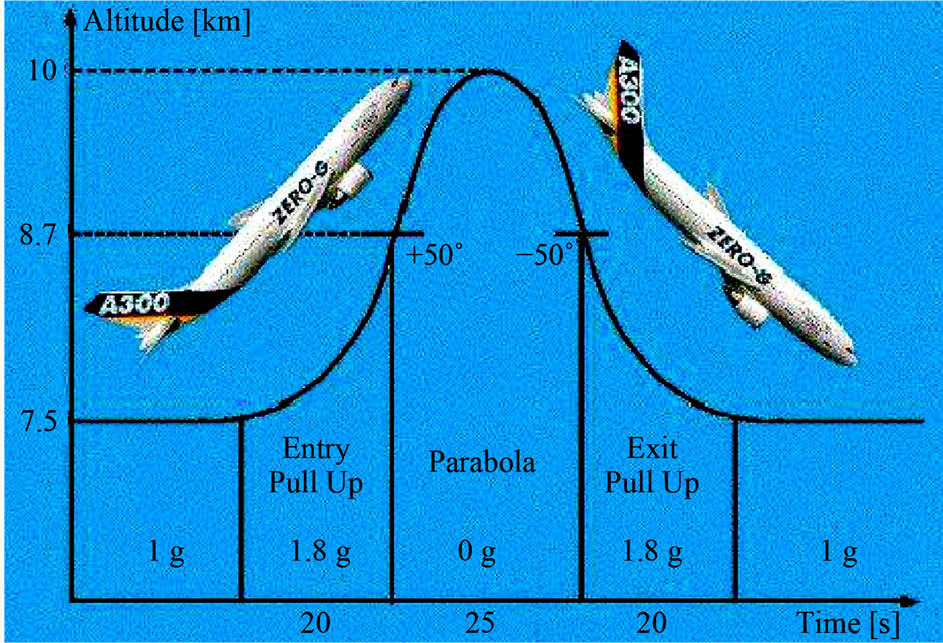
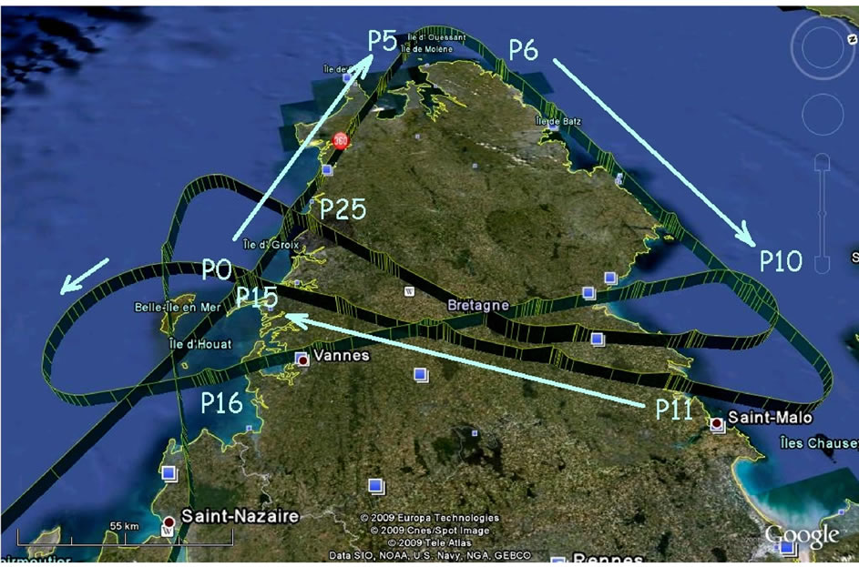
So far, GI-ACs in response to microand hypergravity were monitored during roughly 1000 parabolas and 11 campaigns organized by the DLR and ESA during the years 2002-2012 (Figure 1(a)). During a parabolic flight day 31 parabolas (counting from 0 to 30), are flown consecutively in a time period of about 180 minutes covering a distance of approximately 2200 km. Between single parabolas the airplane flies for two minutes in normal modus (1 × g). After every five parabolas an intermission of about 4 minutes of normal flight occurs before the maneuvers of another five parabolas—generally after directional change—is resumed. Each parabola consists of three phases: 1) 25 s at 1.8 × g (pull-up phase; maximal inclination angle = 47˚), 2) 22 s in microgravity (5 × 10⁻² g, actual parabola), and 3) 25 s at 1.8 × g (pull-out phase, maximal inclination angle of −45˚, i.e. downward flight). During the phases of hypergravity, the g-vector is perpendicular to the floor of the airplane such that persons and objects can stand “normally” as on ground or during horizontal flight. The airplane (Airbus A300- ZERO-G) is located at the international airport of Bordeaux-Merignac and serviced by the company Novespace. The parabolas discussed here were flown over the Atlantic Ocean off the coast of Brittany (cf. Figures 4, 5 and 7).
Figure 1(b) shows the assignment of the three space
 (a)
(a)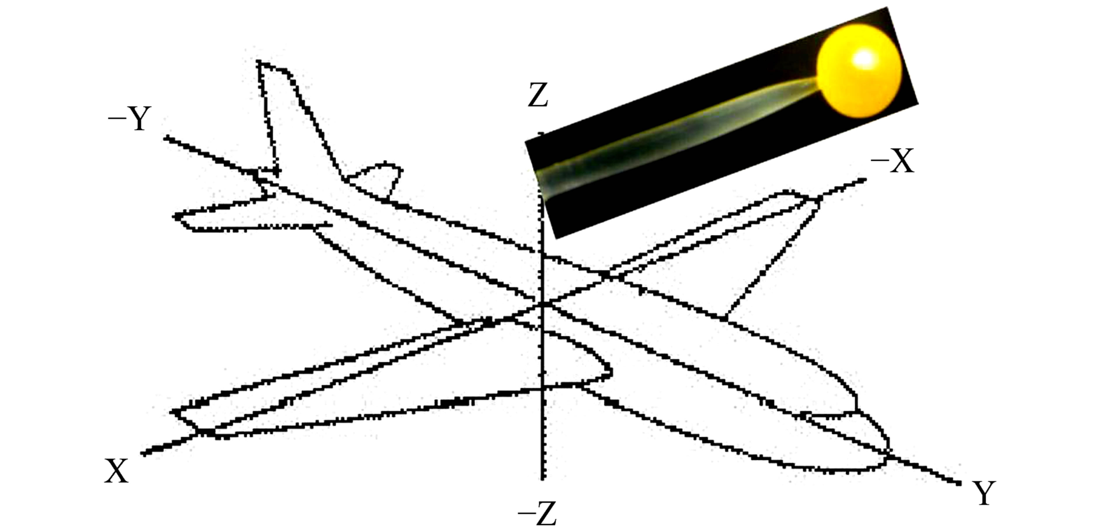 (b)
(b)
Figure 1. (a) Sketch of the path of a single parabola lasting about 3 min, including “pull-up-” and “pullout-maneuvers” lasting 20 to 25 s, and the actual parabola representing 22 to 25 s of weightlessness, for most experimenters the only interesting part. (b) Used assignment of the planes axes, the X-axis measured across the wings, the Y-axis in flight direction and the Z-axis vertical to the planes floor. According to these, the magnetic field sensor monitors the field strength, particularly during parabolas as shown in Figures 3, 4, 6 and 7. The actual position of the SPPHs during all parabolic flights is indicated by the inset photograph.
coordinates. X is the direction across the wings, Y indicates flight direction and Z is the vertical to the planes floor. According to this, both, the three-dimensional Gsensor and the three-dimensional H-sensor (or B-sensor, see below) are fixed and calibrated at the fuselage structure of the plane1.
2.3. Micro Dual Wavelength Spectrometer (MDWS)
Gravity Induced Absorption Changes (GIACs) were detected in vivo with a custom-built micro-dual wavelength spectrometer (MDWS, Figure 2) as described previously [1,2]. Because of the filigree structure of SPPHs (Figure 1(b), inset photograph), we measured reflectance rather than absorption changes as pretended by its name “GIAC”: the relative absorbance A is calculated from the reflected light according to the definition: 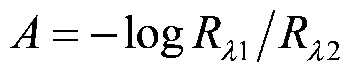 , where R is the reflected light at the wavelengths λ1 and λ2 Without any detriment, in contrast to earlier studies, in the current study we used a much lower chopping frequency of 50 rather than 2000 Hz reducing file size and time of calculations tremendously.
The MDWS (Figure 2) is capable of measuring optical reflection/absorption changes as small as 10−5 to 10−6 A between two wavelengths in a spectral range that is determined by the choice of LEDs (Roithner Lasertechnik, Wien, Austria). Based on the action spectrum of GIACs in the visible wavelength range [3] we selected LEDs in the blue and in the red (λ1 = 460 nm and λ2 = 660 nm). Routinely, the phase of the lock-in amplifier is chosen to deliver an increasing (i.e. upwards) GIACsignal upon increasing absorbance in the blue (i.e. decreasing reflectance), and vice versa. The chopped measuring light beams impinge on the sample and are reflected back to the photomultiplier module (UV-VIS: H5773-01, Hamamatsu Photonics Deutschland GmbH, Herrsching, Germany). A lock-in amplifier (LIA-MV- 200-H; FEMTO Messtechnik GmbH, Berlin, Germany) obtains the reference signal from the LED-control unit and converts the chopped, reflected light stream into the analogues GIAC-signal. This is finally fed to the ADconverter (12 bit AD-DA converter, Intelligent Instruments, UDAS-1001E series, Burr Brown, 10 µs) and then to the notebook (Toshiba, Satellite Pro 4600).
Due to the minute light signals reflected by the thin SPPHs and the maxed out sensitivity of the MDWS the final GIAC signal shows a SNR as small as 5 to 10. The signal of the G-sensor (ADXL105) in the present study only measuring the vertical component of gravitation (Gz)
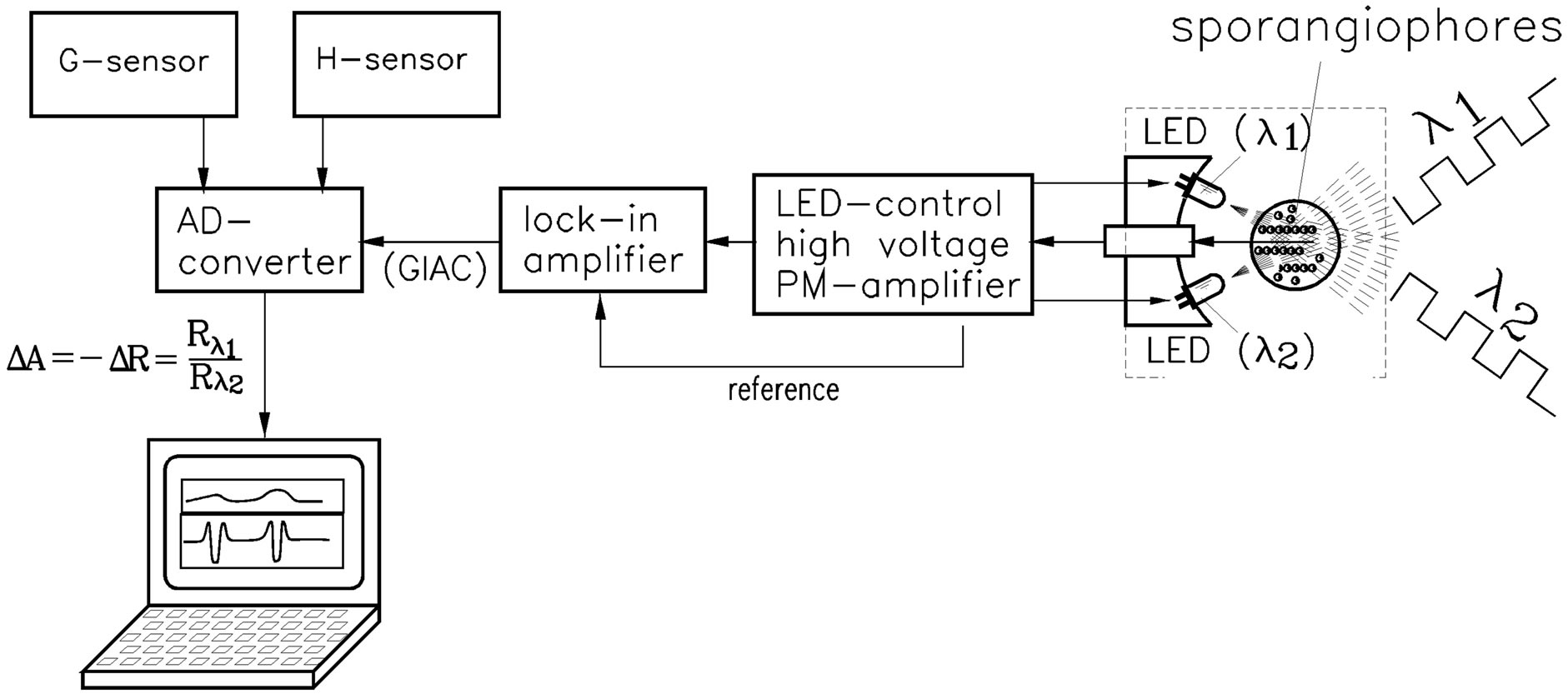
Figure 2. Sketch of the Micro Single Wavelength Spectrometer (MDWS) particularly designed to measure minute absorption/reflection differences. According to the known action spectrum for GIACs (Schmidt, 2006) a red (660 nm) and blue (460 nm) LED were chosen as radiation pair. An electronic generator producing alternating rectangular pulses of 50 Hz which are shifted by 180 degrees alternatively controls both LEDs. Thus, the reflected light stream consisting of alternating pulses of reflected light from the SPPHs is converted to a train of electrical pulses by the mini photomultiplier module. After amplification this is fed to the subsequent lock-in amplifier and converted to an analog difference signal (∆ GIAC). In addition to this the signals of the three-dimensional Gand H-sensors are fed to the analog-digital converter and finally to a laptop. The required reference for the lock-in amplifier is deduced from the chopper electronics.
is also fed to the AD-converter. Both, LEDs and photodetector module are arranged as a compact unit within the measuring box (Figure 2). The components of the MDWS and the organism were kept in a conventional aluminum expedition box (56 cm length × 36 cm width × 41 cm height, about 30 kg) which was fixed to the floor of the airplane. The earth’s magnetic field attains the SPPHs virtually without attenuation.
Even if the dual wavelength method is self-compensating, its extreme sensitivity leads to an inevitable baseline shift. To keep this shift as small as possible, for longer measuring periods as shown in Figures 4, 5 and 7 of more than one hour, sample and MDWS are strictly kept untapped, no adjustments of amplification or baseline corrections are possible. Nevertheless, in some instances our measurements were successful such as in Figures 4-7. Even then, the baseline shift cannot be avoided (see Figure 6(b)) which makes the immediate evaluation difficult. To suppress the still remaining baseline shift of the GIAC kinetics and to place emphasis on the various GIAC-amplitudes observed, a mathematical convolution using an inner (vertical) Z-shaped kernel f(x), Figure 4, was performed, according to the formula:
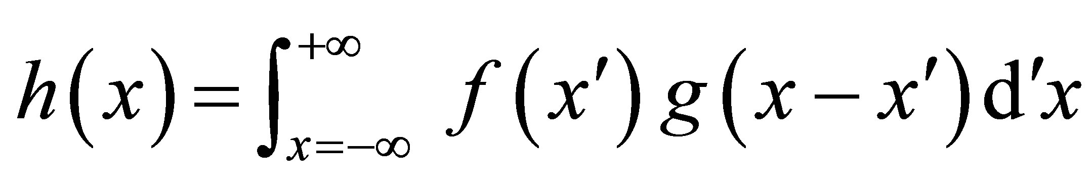 (1)
(1)
 is the so-called “inner kernel”,
  the curve to be convoluted (“folded”) to result in h(x) as shown in the lower part of Figure 6(b). Clearly, a de-
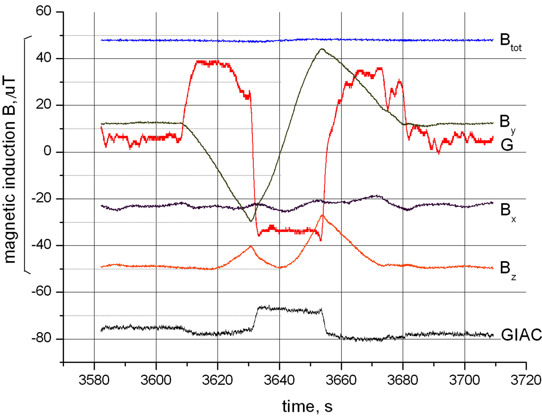
Figure 3. Time course of GIAC, gravity G and various magnetic components as indicated for a single parabola (P12) as measured on 14th Sept 2011. G represents gravitational values in sequence 1 - 1.8 - 0 - 1.8 - 1 g. Bx, By and Bz depict the strength of the three components of the earth’s magnetic field and Btot = 47 µT the calculated total magnetic field.
manding task requiring a fast computer, since each individual point h(x) requires the calculation of a complete integral.
As mentioned above, there is a convenient and simple test for the gravisensitive activity of the sample: The samples (vials) are fixed in a light tight “tilting box”. Its rotation axis is parallel to the y-direction of the plane (Figure 1(b)); thus after tilting by 90˚ the SPPHs are parallel to the x-direction. Tilting of the vertically grown specimen into the horizontal position leads to an (small) intermediate deviation of the measuring signal (∆GIAC, a dummy or “dead” sample does not show this signal). Thus, immediately before the first parabola of a series is flown, we tilt the measuring box by 90 degrees, i.e. position the SPPH in horizontal and active position for the 31 parabolas to come.
2.4. Global Position System (GPS)
The GPS receiver Etrex Vista HCx by Garmin was used to monitor position, altitude, velocity and flight direction of the Airbus 300 Zero G. Every second the data were updated resulting in a densely covered flight path (file type gdb to be imported into Google Earth, Microsoft, via the program Map Source by Garmin). As second, backup GPS-System we used the Minihomer by ZNEX Deutschland (file type gdx to be imported into Google Earth via kmz-file). Both GPS-receivers were placed on a left side window in the rear of the plane receiving strong enough satellite signals allowing continuous monitoring during the whole flight.
Three-dimensional magnetic sensor (H-sensor, Figure
 (a)
(a) (b)
(b)
Figure 4. During the parabolic flights on 9th Feb. 2009 for the first time we selectively searched for the dependency of the GIAC-signal on the flight direction, i.e. the magnetic field of the earth, crossing the peninsula of Brittany. (a) Shows the sequence of three groups of 5 parabolas each, P0 tot P15, each flown in straight direction as indicated in this Google Earth chart representing a complete 360˚ turn. (b) Exhibits the time course of Btot, Bx, the convoluted measureing signal GIACcon and gravity G. The change in flight direction from P0-P5 (315˚) to P6-P10 (50˚) results in the strongest change observed so far (92% increase). To get rid of the shift and to evaluate the various amplitudes observed, a mathematical convolution using a kernel shape as indicated on the right was performed (GIAC-con).
2): Two 3-axis Fluxgate Magnetic Field Sensors FL3-100 (Stefan Mayer Instruments, Dinslaken, Germany) were fixed and calibrated inside the cabin of the plane optionally at two distant positions without remarkable differences. The measurement range for all three components is ±100 µT (delivering ±10 V at each sensor output, accuracy 0.5%). The earth’s magnetic field was not measurably weakened by the planes body (Airbus 300: composed of two aluminum half shells) or the case of the sample-tilting box (Black Trovidur, Polyvinylchloride, PVC).
The total magnetic induction as composed by the three
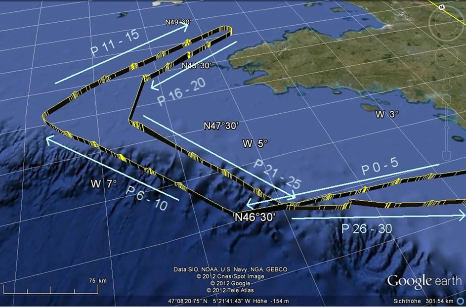
Figure 5. Flight path of the Airbus ZERO G during the parabolic flight campaign (PFC 18) of the DLR on the 14th Sept. 2011 as monitored by the GPS and visualized by Google Earth, off the coast of Brittany. The plane was airborne between 9.33 and 12.23 h in the morning, i.e. roughly 3 hours, covering a distance of 2200 km. Parabolas were flown between altitudes of 6200 and 9200 m (monitored flight profile not shown here). Parabolas are indicated by densely packed vertical yellow lines. Typically, groups of five parabolas are flown in line. Flight direction and the individual parabolas are assigned, resulting in the three components of the magnetic induction of the earth, the total (here from calculated) magnetic induction, and the GIACs as shown in Figure 6(b).
strongly changing components is calculated by
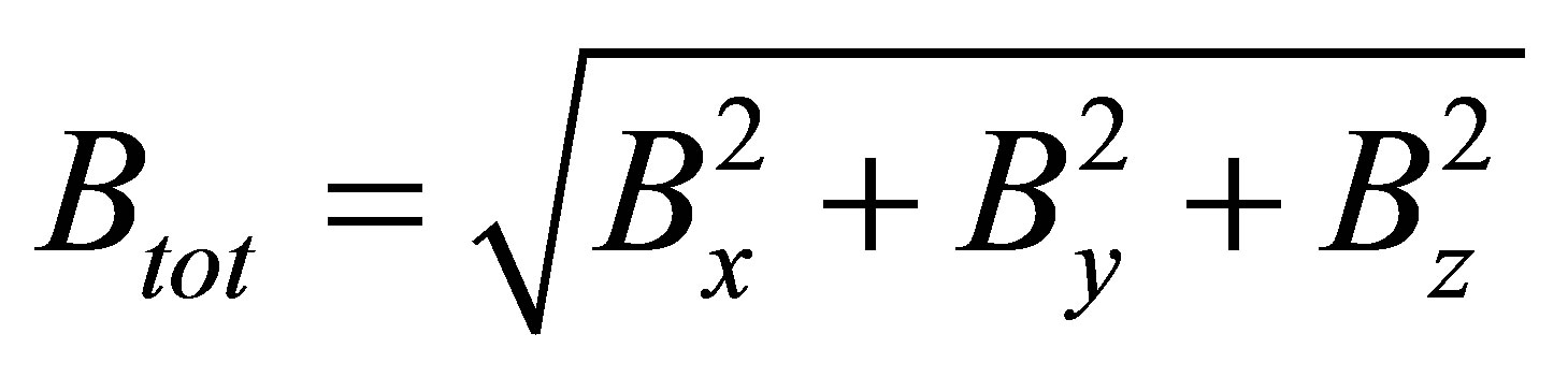 (2)
(2)
In the whole parabolic flight area corresponding to Figures 3-7 (app. Latitude 47˚, longitude −7˚, altitude 8000 m), Btot is essentially constant corresponding to value of Btot = 47 µT according to “British Geological Survey, Geomagnetism”: http://www.geomag.bgs.ac.uk/data_service/models_compass/wmm_calc.html2.
3. Results and Discussion
Time Course of the Three Magnetic Components
The Bx component during any group of 5 parabolas flown in one direction is virtually a flat line with only little variations (Figures 3 and 6). However, upon directional change this component shifts significantly (Figures 4, 6 and 7). Rotation of the plane around the x-axis (across the wings, Figure 1) during the parabolas does not influence this signal. The small variations simply reflect wiggling of the plane around the yand z-axes, i.e. imperfection of flight. The Bx component essentially represents the azimuth angle of the flight path.
The By component is oriented in the lengths axis of the plane (Figure 1) and shows a kind of saw tooth shape
 (a)
(a)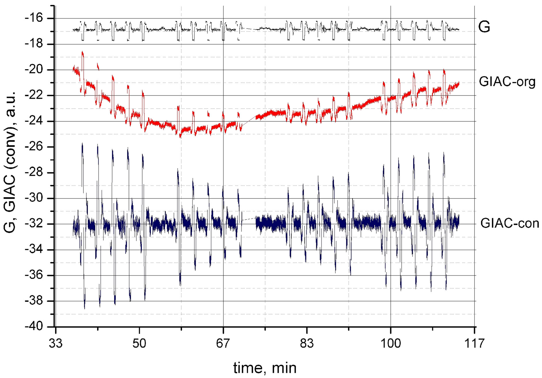 (b)
(b)
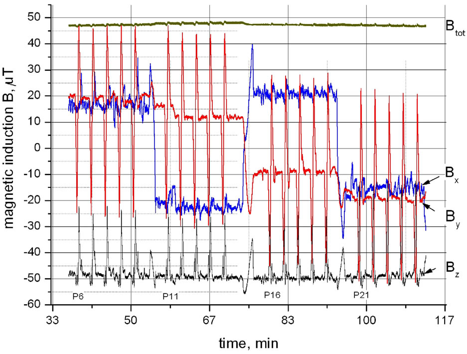
Figure 6. Similar to Figure 4, parabolas P6 to P25 which represent a sequence of four groups covering an angle of approximately 180˚. (a) Survey of all three components of the magnetic field as measured in μT. Blue: Bx, red By and grey Bz component. The upper straight red line represents the calculated total magnetic field Btot = 47 µT. (b) (a.u.): black upper curve time course of G. Red middle curve represents the original GIAC-signal (GIACorg), blue lower curve convoluted GIAC-kinetics.
 (a)
(a)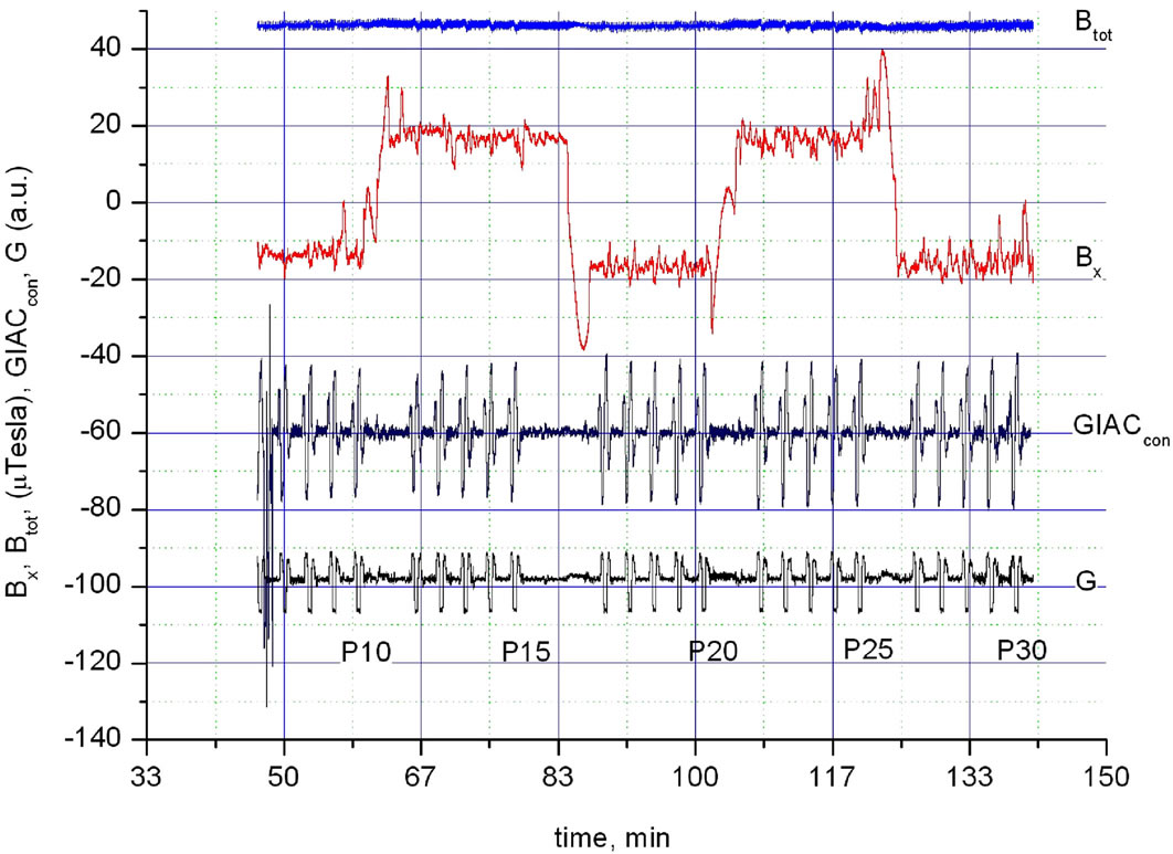 (b)
(b)
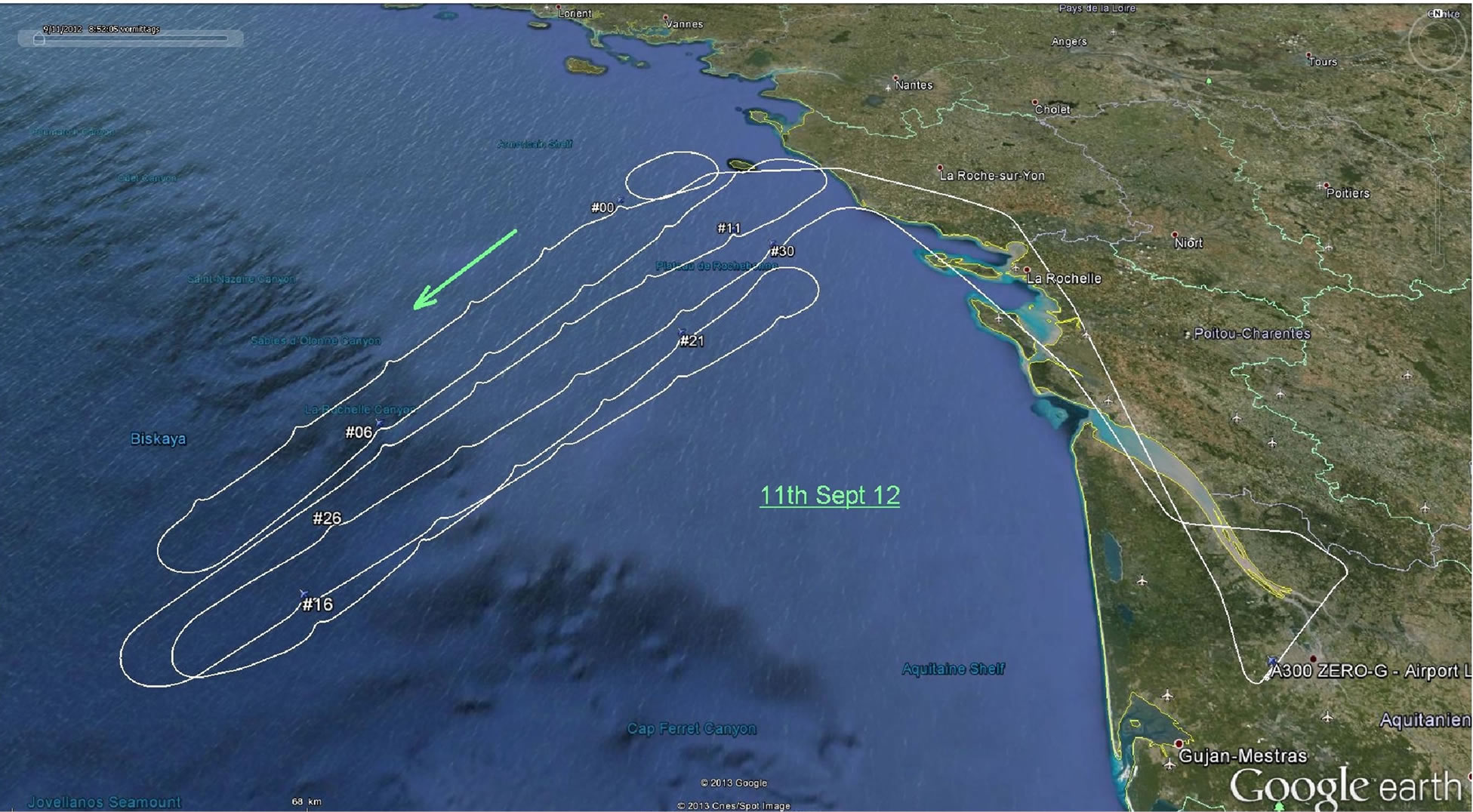
Figure 7. The next experiment flown on 11th Sept. 2012 was technically perfect with excellent samples and little baseline shift, yielding a good GIAC-signal. Top: Unfortunately, all parabolas flown on 11th Sept 2012 are directed approximately to the same or reverse direction (244˚ resp. 64˚) giving rise to nearly identical GIAC-signals. Therefore, this flight day was not very informative but confirms the validity of the experiment and the expected constancy of GIACs.
with more or less connecting straight lines. The longer middle line connecting the corners of lowest and highest field values represents the parabola itself, i.e. time of weightlessness of 22 s (Figure 3). This is simply explained by the fact that the first derivative of the parabolic path/time course is a straight line. Deviation of the straightness is a measure of imperfection of the parabola. The straight lines during hypergravity during the pull-up and pull-out maneuvers also reflect (reverse) parabolic parts of the flight path.
The Bz component shows a characteristic double corner during parabolas but remains on the same level for all flight directions. The explanation is similar to that of the By component. The two corners enclose the period of weightlessness. In the Atlantic area flown (Figure 3) at a height of 8000 m the earth’s magnet field lines impinge in an inclination angle between 59 to 63 degrees (see inclination/declination calculator): http://www.geomag.bgs.ac.uk/data_service/models_compass/wmm_calc.html.
During any parabola and depending on flight direction the plane intersects these lines under various angles resulting in the observed sharp “double corner” of the Bz component with varying height of the two corners (Figure 6(a)).
During the parabolic flights on 9th Feb. 2009 for the first time we selectively searched for the dependency of the GIAC-signal on the flight direction crossing the peninsula of Brittany. Figure 4(a) shows the sequence of three groups of 5 parabolas P0 tot P15 each flown in straight direction as indicated in this Google Earth chart representing a complete 360˚ turn. Figure 4(b) exhibits the time course of Htot, Hx, GIACcon and gravity G. The change in flight direction from P0-P5 (315˚) to P6-P10 (50˚) shows the most dramatic effect observed so far (92% increase).
The set of parabolas P6 to P25 flown on 14th Sept 2011 (Figure 5) present a unique example of GIAC-changes upon nearly reverted and orthogonal flight passes. Figure 6(a), shows the time course of Btot and of all three magnetic components Bx, By and Bz. Figure 6(b), shows gravity (G), the original GIAC-signal (GIACorg) and the convoluted i.e. shift-free GIAC signal (GIACcon). Interestingly, the GIAC signal does not change instantaneously upon directional change (P6-P10 to P11-P15) or (P11-P15 to P16-P20) but exhibits some kind of adaptation, i.e. a slow change with the new magnetic situation, i.e. direction. Slow adaptive processes are well known in plant physiology, even if badly understood [15].
The next experiment shown was technically successful with excellent samples, yielding a good GIAC-signal. Unfortunately, all parabolas flown on 11th Sept 2012 are directed approximately to the same or reverse direction (244˚ resp. 64˚) giving rise to nearly identical GIACsignals (GIACcon, Figure 7). Therefore, this flight day was not very informative, however confirms the validity of the experiment and the expected constancy of GIACs.
4. Conclusion and Related Phenomena
In this context, very puzzling phenomena related to magneto reception need to be mentioned: Caryopses (grains) of various specimen such as Avena sativa, Hordeum vulgare, Secale cereale and seeds of flax when oriented parallel to the earth’s magnetic field germinate and grew faster than those with perpendicular orientation [16,17]. Enhanced germination of caryopses occurres in Zea mays and Triticum aestivum when the roots are oriented towards the south pole [18]. However, not all plant species have the capacity for magneto orientation [19], so far no magneto responses are known in Phycomyces (Galland, personal information). In addition, clear-cut biological responses to geomagnetic storms of the sun have been described, even if fluctuations of the Earth’s magnetic field are extremely small as 500 nT [20]. Still more puzzling: Clockwise rotation of Avena sativa caryopses retarded the elongation growth of coleoptiles and roots, while a counterclockwise rotation caused an enhancement [21]. Except for the various forms of orientation of mammals, migrating birds and microorganisms, so far, no biological advantage of any other magneto response is immediately obvious. Thus, most studies as the present one remain largely on a phenomenological level and typically lack mechanistic insight.
5. Acknowledgements
The work was supported by grant BW 1025 from the DLR/BMBF (Deutsches Zentrum für Luftund Raumfahrt, and Bundesministerium für Bildung und Forschung). First of all, I thank my college Prof. Galland for many discussions of these GIAC experiments. We are greatly indebted to the members of the electronic and machine shops of the biology department of the University of Marburg, first and foremost Manfred Peil, as well as Herbert Mootz, Sebastian Richter, Eric Schnabel and Andreas Gerber, who constructed and build the MDWS. We thank Marco Goettig for excellent technical assistance.
REFERENCES
- W. Schmidt, Journal of Biochemical and Biophysical Methods, Vol. 58, 2004, pp. 15-24. http://dx.doi.org/10.1016/S0165-022X(03)00153-2
- W. Schmidt, Microgravity-Science and Technology, Vol. 19, 2007, pp. 11-15. http://dx.doi.org/10.1007/BF02870983
- W. Schmidt, Protoplasma, Vol. 229, 2006, pp. 125-131. http://dx.doi.org/10.1007/s00709-006-0217-8
- W. Schmidt and P. Galland, Planta, Vol. 210, 2000, pp. 848-852. http://dx.doi.org/10.1007/s004250050689
- W. Schmidt and P. Galland, Plant Physiology, Vol. 135, 2004, pp. 183-192. http://dx.doi.org/10.1104/pp.103.033282
- W. Schmidt, Microgravity Science and Technology, Vol. 22, 2010, pp. 79-85. http://dx.doi.org/10.1007/s12217-009-9113-0
- J. D. Palmer, Nature, Vol. 198, 1963, pp. 1061-1062. http://dx.doi.org/10.1038/1981061a0
- C. David and K. Easterbrook, The Journal of Cell Biology, Vol. 48, 1971, pp. 15-28. http://dx.doi.org/10.1083/jcb.48.1.15
- R. Blakemore, Science, Vol. 190, 1975, pp. 377-379. http://dx.doi.org/10.1126/science.170679
- E, Wajnberg, D. Acosta-Avalos, O. C, Alves, J. Ferreira de Oliveira, R. B. Srygley and D. M. S, Esquivel, Journal of the Royal Society Interface, Vol. 7, 2010, pp. 207-225.
- H. Nicol and M. Locke, Science, Vol. 29, 1995, pp. 1888- 1889. http://dx.doi.org/10.1126/science.269.5232.1888
- J. L. Kirschvink and J. L. Gould, Biosystems, Vol. 13, 1981, pp. 181-201. http://dx.doi.org/10.1016/0303-2647(81)90060-5
- T. Ritz, P. Thalau, J. B. Phillips, R. Wiltschko and W. Wiltschko, Nature, Vol. 429, 2004, pp. 177-179. http://dx.doi.org/10.1038/nature02534
- A. Pazur, C. Schimek and P. Galland, Central European Journal of Biology, Vol. 2, 2007, pp. 597-659. http://dx.doi.org/10.2478/s11535-007-0032-z
- W. G. Hopkins and N. P. A. Huner, “Introduction to Plant Physiology,” 4th Edition, APS Press, 2012, 528 p.
- U. J. Pittman, Biomedical Sciences Instrumentation, Vol. 1, 1963, pp. 117-122.
- U. J. Pittman, Canadian Journal of Plant Science, Vol. 42, 1962, pp. 430-436. http://dx.doi.org/10.4141/cjps62-070
- A. V. Krylov and G. A. Tarakanova, Plant Physiology, Vol. 7, 1960, pp. 156-160.
- P. Galland and A. Pazur, Journal of Plant Research, Vol. 118, 2005, pp. 371-389. http://dx.doi.org/10.1007/s10265-005-0246-y
- E. R. Nanush’yan and V. V. Murashew, Russian Journal of Plant Physiology, Vol. 50, 2003, pp. 522-526.
Abbreviations
DLR: Deutsches Zentrum für Luftund Raumfahrt;
ESA: European Space Agency;
GIAC: Gravity Induced Absorption Change;
Google Earth: Virtual Globe; converts GPS data for 3D visualization;
GPS: Global Positioning System;
LIAC: Light Induced Absorption Change;
MDWS: Micro Dual Wavelength Spectrometer;
PFC: Parabolic Flight Campaign;
SNR: Signal to Noise Ratio;
SPPH: Phycomyces sporangiophore (carrying app. 106 spores each).
NOTES
1As commonly used, bearings are always calculated based on north being zero degrees, and degrees are then counted moving clockwise around the circle of 360˚ from there.
2Often the terms magnetic field H, magnetic induction B, magnetic fluxor -flow density, are used deliberately in confusing manner, particularly throughout the biological magneto-related literature. The magnetic field H is physically defined by the force experienced by a closed current loop [A/m]. The French physicist A. Ampère (1775- 1836) originated the idea that there are micro-currents in each body generated by the motion of electrons in atoms and molecules. These molecular currents produce their own magnetic field. The interaction of these micro-fields Hm and the external field H results in the magnetic flux density or magnetic induction B [kg∙m∙A−1∙s−2], (SI-units), shortly termed “Tesla” (T). Thus, B and H are proportional according to the equation B = μ0μH, with μ0,SI [4π ×10−7 Vs/Am] as the permeability of the vacuum, and the dimensionless relative permeability μ (a tensor!) indicates of how much the external field is amplified by the micro currents of the specific material (μ = 1 for the vacuum or air). If the external field H overrides the internal “micro currents” we observe saturation and the typical “magnetization curve” (B vs. H) runs parallel to the vacuum curve. Thus, following general linguistic usage and keeping the proportionality of B and H in mind, as long as µ = 1 as in our case for air, we use the terms “magnetic induction” and “earth’s magnetic field” optionally, even if generally measured in units of “Tesla”.