Journal of Modern Physics
Vol.3 No.11(2012), Article ID:24854,6 pages DOI:10.4236/jmp.2012.311223
Hough Transform to Study the Magnetic Confinement of Solar Spicules
1Physics Department, Payame Noor University, Tehran, Iran
2Institut d’Astrophysique de Paris, Paris, France
3Center for Excellence in Astronomy & Astrophysics (CEAA-RIAAM ), Maragha, Iran
Email: etavabi@yahoo.com, koutchmy@iap.fr, ali_ajabshir@yahoo.com
Received September 1, 2012; revised October 1, 2012; accepted October 13, 2012
Keywords: Solar Chromosphere; Spicule; Hough Transform; Tracing; Magnetic Focusing
ABSTRACT
One of the important parameters of the ubiquitous spicules rising intermittently above the surface of the Sun is the variation of spicule spline orientation with respect to the solar coordinates, presumably reflecting the focusing of ejection by the coronal magnetic field. Here we first use a method of tracing limb spicules using a combination of second derivative operators in multiple directions around each pixel to enhance the visibility of fine linear part of spicules. Furthermore, the Hough transform is used for a statistical analysis of spicule orientations in different regions around the solar limb, from the pole to the equator. Our results show a large difference of spicule apparent tilt angles in regions of: 1) the solar poles, 2) the equator, 3) the active regions and 4) the coronal holes. Spicules are visible in a radial direction in polar regions with a tilt angle <20˚. The tilt angle is even reduced inside a coronal hole (open magnetic field lines) to 10 degrees and at the lower latitude the tilt angle reaches values in excess of 50 degree. Usually, around an active region they show a wide range of apparent angle variations from –60 to +60 degrees, which is in close resemblance to the rosettes made of dark mottles and fibrils seen in projection with the solar disk.
1. Introduction
The origin of the upper levels of the solar atmosphere heating and the fast wind mass loss seem directly related to the dynamic behavior of the solar spicules or of regions directly above having a more extended structure, the so-called giant or macro-spicules and spikes. References [1] and [2] directly relate spicule orientation to the ambient coronal magnetic field and Auchere et al. claimed that it could be related to the chromosphere prolateness effect [3]. Reference [4] claimed a relation between inclinations of magnetic flux tubes and the tunneling of low-frequency photospheric P-modes which are more than sufficient in carrying energy fluxes into the corona and transition region. Less than one percent of the spicule mass is indeed transported towards the corona and this is enough to compensate for solar fast wind mass losses located in coronal holes, see [5] and [6], where the spicules are more vertical and taller than the quieter solar spicules. Giant and macro spicules are believed to sometimes give an EUV and SXR (Soft X-Ray) jet which could be explained in case of a release of sufficient energy coming from the free energy of the coronal magnetic field [7] and related to process occurring near a magnetic null point, including reconnection events.
Several authors have listed the physical parameters of spicules [8-12] and others based on off-disk measurements of projected linear structures at a known true angle with respect to the solar local vertical [13,14].
They found that the most common inclination is in the range of 20 - 45 degrees and the average true inclination is about 36 degrees for measurements made below the 70˚ latitude. These are somewhat broader than the distributions found by Beckers [9] who found a variation from the vertical of 20 degrees at a 60˚ latitude. Van de Hulst [15] could not specify the average orientation. Reference [16] found the average inclination around the axis of symmetry is 29 degrees and that the average spicule tends to be inclined toward the equator. More recently, Pasachoff recorded measurements near the solar minimum activity and found a tilt of 27 degrees with a 5 degrees dispersion, while Heristchi and Mouradian’s measurements were taken in 1970 at solar maximum.
The orientation of spicules is a valuable parameter in absence of direct magnetic field measurements of sufficient resolution in this region, because it is presumably determined by the flow of plasma which should occur along the magnetic field lines, especially where the solar magnetic field pressure dominates the gas pressure.
Of course, all these measurements suffered from overlapping effect of spicules seen along each line of sight, the effect of which will be more important when we look near the solar limb, see reference [17] for a model investtigation of this effect.
The main purpose of this paper is to automatically and objectively determine the apparent tilt angle of spicules spline using excellent observations from the seeing free Solar Optical Telescope (SOT) limb imaging experiment, [18,19], onboard Hinode [20]. A technique for the automatic detection of limb spicules has been developed and statistical measurements were conducted for determining the tilt angle for spicules at different heliocentric angles.
2. Observations and Data Reduction
We selected five sequences of solar limb observations made at different positions of the limb using the broadband filter instrument (BFI) of the SOT of the Hinode mission (Table 1). We use series of image sequences obtained in the Ca II H chromospheric and still “cool” emission line; a wavelength pass-band centered at 398.86 nm with a FWHM of 0.3 nm and a cadence of 20 seconds is used with an exposure time of 0.5 s giving a spatial resolution of the SOT-Hinode limited by the diffraction at 0"16 or 120 km on the Sun; a 0"0541 pixel size scale is used.
We used the SOT routine program “fg_prep” to reduce the image parasitic spikes and the jitter effect and to align the time series. The time series show a slow pointing drift, with an average speed less than 0’’015/min toward the north as illustrated by the very slow solar limb motion.
A superior spatial image processing for thread-like features is obtained using the mad-max algorithm [21] and [22]. See Figure 1 and top panels of Figures 2 and 3 for ex. Table 1 illustrates information on all positions and dates (first and second columns) which are used in this paper. The size of each image used is 1024 × 512 pixels2 (Hinode read out only the central pixels of the larger detector to keep the high cadence within the telemetry restrictions) thus covering an area of (FOV) 111" × 56".
For the detection and tracing of spicules in 2D we apply and develop a method with the following steps: 1) To increase the visibility of spicules, a radial logarithmic scale is applied; 2) To enhance linear features, the Madmax operator is used [22]. The aim of the Madmax operator is to trace the bright hair-like features in solar ultimate observations polluted by a noise of different origins. This popular spatial operator uses the second derivative in an optimally selected direction for which its absolute value has a maximum value (Figure 1).
Figure 1 shows an example of these processing made to avoid artifact effects due to compression or calibration. We use the raw data, but still some artifacts related to pixel size and to the transformation methods are seen; note also the CCD read-out defect near the center of the frames in Figure 2.
Next, we consider the spicule apparent inclinations using the Hough transform (Hough, 1962). This section describes how to use the Hough transform functions to detect lines in an image. This transformation method is a feature extraction technique that finds imperfect instances of objects within a certain class of shapes. The simplest case of Hough transform is the linear transform for detecting straight lines. The Hough transform creates an accumulator matrix. The (r,θ) pair represents the location of a cell in the accumulator matrix. Every valid (logical true) pixel of the input binary image (xi, yj) represented by (R,C), produces a r value for all θ values (see Figure 4). The block quantifies the r values to the nearest number in the r vector. The r vector depends on

Table 1. Observational parameters.
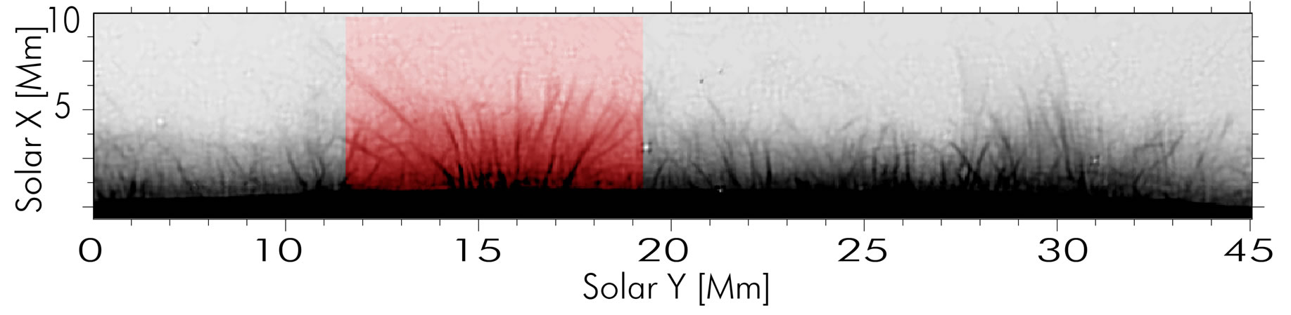
Figure 1. Negative and processed image taken on 2008- 09-09; the highlighted region will be shown in Figure 4 again.
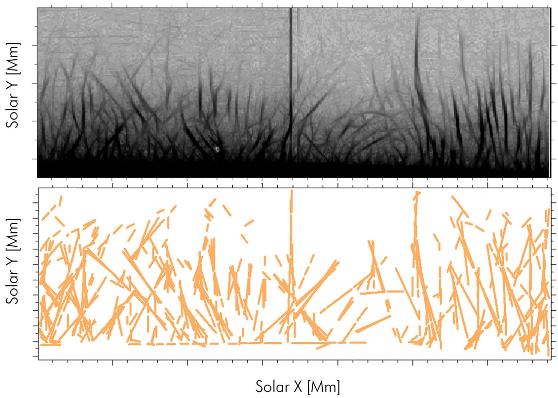
Figure 2. At top: negative and processed image taken on 2011-06-17; at bottom: result of line tracing using the Hough transform. The strictly vertical dark line near the center was caused by the CCD readout system.

Figure 3. At top: negative and processed image taken on 2008-09-09 (sub-frame and highlighted section of Figure 1); bottom: a result of line tracing using the Hough transform.
the size of the input image and the user-specified r resolution. The block increments a counter (initially set to zero) in those accumulator array cells represented by (r, θ) pairs found for each pixel, the straight line can be described as yj = Rxi + C. This process validates the point (R,C) to be on the line defined by (r, θ). The block repeats this process for each logical true pixel in the image (Figure 4). The Hough outputs the resulting accumulator matrix. If the curves corresponding to two points are superimposed, the location (in the Hough space) where they cross
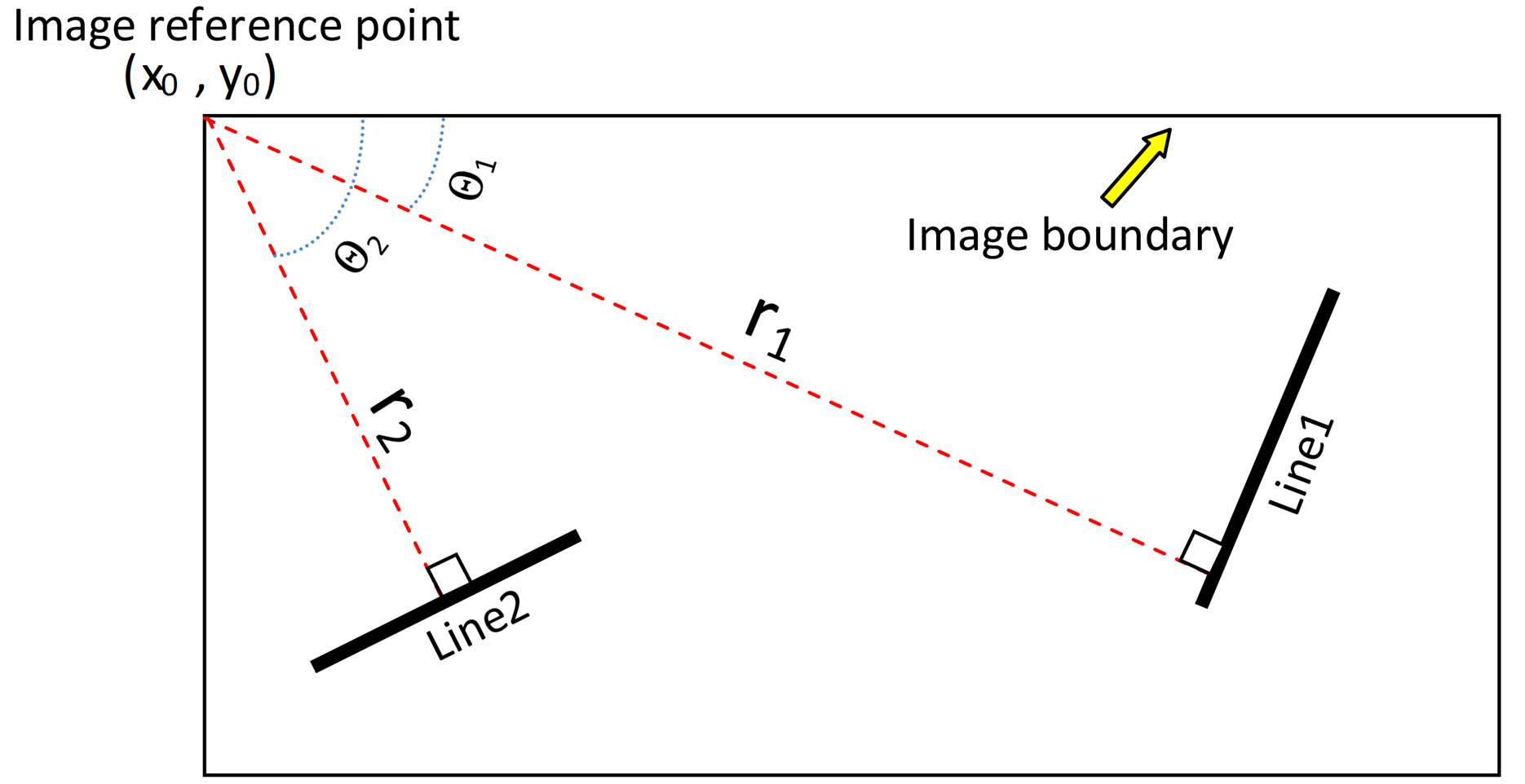
Figure 4. Schematic to show line 1 and line 2 and the boundary of the reference image.
corresponds to a line (in the original image space) that passes through both points. More generally, a set of points that form a straight line will produce sinusoids which cross at the parameters for that line [23].
The classical Hough transform concerned the identifycation of lines in images, but nowadays the use of the Hough transform has been extended to identifying positions of arbitrary shapes, most commonly loops and ellipses. Thus, it is an ideal method to find all linear structures. To qualify them as a spicule, we started assuming they must be longer than 2" (~20 pixels for SOT).
Figures 2 and 3 show a result of line segmentation using the Hough transform. With this transformation we can trace more than 70 percent of spicules, when visually comparing mad-maxed image and the Hough transformed data. In Hough transformation this rate could be increased by changing the segmentation value qualifying features as spicules. Finally, spicules were defined as bright and straight features which are more than 2 arcsec (about 20 pixels) long and at least 4 pixels wide. Using these values we obtained a typical level of accuracy of about 70 percent, although in several cases, at crossing points, such accuracy could not be found. The average value for spicule length is about 5000 to 10,000 km and they have a wide range of widths (in close agreement with Tavabi et al. [12]).
The tilt angle distribution of the fine H Ca II spicules is exactly the same in both directions left and right from the normal direction with an absolute value of about 50 degrees. This behavior is shown by the spicule tracing using the Hough transform in Figure 3, and the matrix of the Hough transform clearly showing a statistically equal tilt angle (red color in panel (b) of Figure 5).
3. Results
We investigated the apparent inclination of spicules and found a statistically average value for different locations around the solar limb. All these results are outlined in Table 1 for four of them (minimum activity), and the Hough matrix elements are plotted in Figure 5.
These results are indeed in general agreement with Pa-
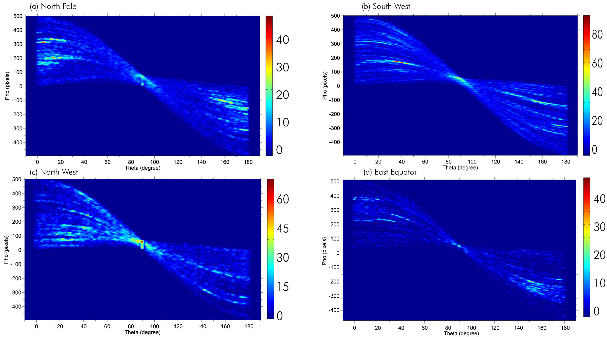
Figure 5. The matrix of Hough transformations for different heliocentric positions as outlined in Table 1. The x-axis shows the inclination angle. The vertical axis shows the distance of spicules from the top left corner of the image (see Figure 2), which is the reference point of the image (0, 0) in Cartesian coordinates. The right color bars give the corresponding number of detected spicules.
sachoff [11] and Heristchi and Mouradian [16]. We however found a big difference between polar region angles for the quiet Sun and for the coronal hole region of the active Sun (Figure 5), when the B angle had a large value and when the coronal hole layers were visible (Figure 2). In this figure, spicules are mostly taller and radial; in addition, some small loops were also seen there.
The quiet Sun spicules in the lower latitude were oriented in a direction pointing toward the solar equator. This behavior had been reported by Heristchi and Mouradian [16]. But Pasachoff et al. [11] could not find such correlation. In our study, we found that this effect depends on the activity of the nearby region; in this case it is at North East in Figure 6. A large difference was seen between the two opposite directions as a result of the presence of active regions. To confirm this effect, we would need a larger field of view. The Hough transform matrix also gives us a rough estimate of the number of detected spicules (or straight lines) over the image (Table 1, column 3 and the corresponding color bar for each plot).
4. Discussion and Conclusion
The solar chromosphere above 1.5 Mm or even less is not exactly a spherically stratified atmosphere as assumed in classical hydrostatic atmospheric models. The upper edge of the chromosphere seen at moderate resolution in strong chromospheric emission lines is rather “blurred” as it consists of the mixture of a large number of jet-like dynamic spicules and of coronal plasma between them. Many past observations showed that at the epoch of solar minimum the extension of the chomosphere near the poles is systematically higher than at the equator ([3,24,25]) and modern precise measurements confirmed and substantiated these early suggestions ([1,26]). The amount of prolateness depends of phase of the solar cycle, of the behavior of spicules and possibly of the inter-spicule matter. The difference in the height of polar and equatorial chromospheres arises due to the difference in structure of polar and low latitude magnetic fields. It is well-known that the large-scale magnetic field in polar regions is mostly open at the sunspot minimum, while in the equatorial region it is mostly closed according to the dominance of the global dipolar and octupolar spherical harmonics. The small-scale structure of the magnetic field in the two regions is likely not being the same. The real fine structure of the polar magnetic field is elusive. There is a strong suspicion that it is very similar to the fine structure of the magnetic field within coronal holes sometimes observed at low latitudes. As far as we know, the chromospheric layer is mainly filled with spicules and the thickness of the chromosphere shows a

Figure 6. Matrix of the Hough transform for the South Pole coronal hole of 2011 June 17 corresponding to the last row of data (e) which was shown in Table 1.
wide range of variations (from pole to equator and quiet to active Sun during the solar cycle). This has been reported by several authors ([1,3,27]). They have suggested that the elevation of the limb in the chromosphere may be caused by the presence of spicules. The polar extension seems consistent with a reduced heat input to the chromosphere in the polar coronal holes compared to the quiet-Sun atmosphere at the equator vs. the active-Sun. However, a strong link to the local magnetic field determines the direction of spicules and their focusing. The falling back of the spicule material due to the solar gravity attraction is feeding the interspicular space that is more diffuse and possibly hotter. The result of our analysis points to a specific relationship of the spicule directions and the spicule/interspicule magnetic topology that could be more easily evidenced using observations made in hotter emission lines. This should be now studied thanks to the data made recently available from the AIA experiment of the SOT mission of NASA.
5. Acknowledgements
We are grateful to the Hinode team for their wonderful observations. Hinode is a Japanese mission developed and launched by ISAS/JAXA, with NAOJ as a domestic partner and NASA, ESA and STFC (UK) as international partners. This work has been supported by the Iran National Foundation (INSF) that E.T. gratefully acknowledges. This work has been supported financially by Center for Excellence in Astronomy & Astrophysics (CEAARIAAM ) under research project No. 1/2643. The image processing OMC software (often called Madmax) written for IDL is easily downloadable from the O. Koutchmy site at UPMC, see http://www.ann.jussieu.fr/~koutchmy/ debruitage/madmax.pro.
REFERENCES
- B. Filippov and S. Koutchmy, “On the Origin of the Prolate Solar Chromosphere,” Solar Physics, Vol. 196, No. 2, 2000, pp. 311-320. doi:10.1023/A:1005296100860
- P. Lorrain and S. Koutchmy, “Two Dynamical Models for Solar Spicules,” Solar Physics, Vol. 165, No. 1, 1996, pp. 115-137. doi:10.1007/BF00149093
- F. Auchere, S. Boulade, S., Koutchmy, R. N. Smartt, J. P. Delaboudiniere, A. Georgakilas, J. B. Gurman and G. E. Artzner, “The Prolate Solar Chromosphere,” Astronomy & Astrophysics, Vol. 336, 1998, pp. L57-L60.
- B. De Pontieu, R. Erdelyi and S. P. James, “Solar Chromospheric Spicules from the Leakage of Photospheric Oscillations and Flows,” Nature, Vol. 430, No. 6999, 2004, pp. 536-539. doi:10.1038/nature02749
- G. Athay, In: P. A. Sturrock, Ed., Physics of the Sun, Reidel Publishing, Norwell, 1986.
- K. Wilhelm, L. Abbo, F. Auchère, N. Barbey, L. Feng, A. H. Gabriel, S. Giordano, S. Imada, A. Llebaria, W. H. Matthaeus, G. Poletto, N. E. Raouafi, S. T. Suess, L. Teriaca and Y. M. Wang, “Morphology, Dynamics and Plasma Parameters of Plumes and Inter-Plume Regions in Solar Coronal Holes,” The Astronomy and Astrophysics Review, Vol. 19, No. 1, 2011, p. 35. doi:10.1007/s00159-011-0035-7
- B. Filippov, S. Koutchmy and E. Tavabi, “About the Magnetic Origin of Chromospheric Spicules and Coronal Jets,” Solar Physics, 2012. doi:10.1007/s11207-011-9911-6
- Z. Mouradian, “Contribution à l’étude du Bord Solaire et de la Structure Chromospherique,” Annales d’Astrophysique, Vol. 28, 1965, p. 805
- J. M. Beckers, “Solar Spicules,” Solar Physics, Vol. 3, No. 3, 1968, pp. 367-433.
- A. C. Sterling, “Solar Spicules: A Review of Recent Models and Targets for Future Observations, Solar Spicules,” Solar Physics, Vol. 196, No. 1, 2000, pp. 79-111. doi:10.1023/A:1005213923962
- J. M. Pasachoff, A. J. William and A. C. Sterling, “Limb Spicules from the Ground and from Space,” Solar Physics, Vol. 260, No. 1, 2009, pp. 59-82. doi:10.1007/s11207-009-9430-x
- E. Tavabi, S. Koutchmy and A. Ajabshirzadeh, “A Statistical Analysis of the SOT-Hinode Observations of Solar Spicules and Their Wave-Like Behavior,” New Astronomy, Vol. 16, No 4, 2011, pp. 296-305. doi:10.1016/j.newast.2010.11.005
- J. M. Mosher and T. P. Pope, “A Statistical Study of Spicule Inclinations,” Solar Physics, Vol. 57, No. 2, 1977, pp. 375-384. doi:10.1007/BF00160281
- S. Koutchmy and M. L. Loucif, “Properties of Impulsive Events in a Polar Coronal Hole (With 6 Figures),” In: P. Ulmschneider, E. R. Priest and R. Rosner, Eds., Mechanisms of Chromospheric and Coronal Heating, SpringerVerlag, Berlin, 1991, p. 152.
- H. C. Van de Hulst, “The Sun,” University of Chicago Press, Chicago, 1953.
- D. Heristchi and Z. Mouradian, “On the Inclination and the Axial Velocity of Spicules,” Solar Physics, Vol. 142, No. 1, 1992, pp. 21-34. doi:10.1007/BF00156631
- E. Tavabi, S. Koutchmy and A. Ajabshirzadeh, “Contribution to the Modeling of Solar Spicules,” Advances in Space Research, Vol. 47, No. 11, 2011, pp. 2019-2029. doi:10.1016/j.asr.2011.01.023
- S. Tsuneta, K. Ichimoto, Y. Katsukawa, et al., “The Solar Optical Telescope for the Hinode Mission: An Overview,” Solar Physics, Vol. 249, No. 2, 2008, pp. 167-196. doi:10.1007/s11207-008-9174-z
- Y. Suematsu, K. Ichimoto, Y. Katsukawa, T. Shimizu, T. Okamoto, S. Tsuneta, T. Tarbell and R. A. Shine, “High Resolution Observations of Spicules with Hinode/SOT,” Astronomical Society of the Pacific, Vol. 397, 2008, p. 27.
- T. Kosugi, K. Matsuzaki, T. Sakao, T. Shimizu, Y. Sone, S. Tachikawa, T. Hashimoto, et al., “The Hinode (Solar-B) Mission: An Overview,” Solar Physics, Vol. 273, No. 1, 2007, pp. 3-17. doi:10.1007/s11207-007-9014-6
- O. Koutchmy and S. Koutchmy, “Optimum Filter and Frame Integration: Application to Granulation Pictures,” Proceedings of 10th Sacramento Peak Summer Workshop, High Spatial Resolution Solar Observations, New Mexico, 22-26 August 1988, p. 217.
- E. Tavabi, S. Koutchmy and A. Ajabshirizadeh, “Increasing the Fine Structure Visibility of the Hinode SOT Ca (ii) H Filtergrams,” Solar Physics, 2012, in Press.
- L. Shapiro and G. Stockman, “Computer Vision,” Prentice-Hall, Inc., New York, 2001.
- A. J. Secchi, “Le Soleil,” Gauthier-Villars, Paris, 1877.
- W. O. Roberts, “A Preliminary Report on Chromospheric Spicules of Extremely Short Lifetime,” The Astrophysical Journal, Vol. 101, 1945, pp. 136-140. doi:10.1086/144699
- A. Johannesson and H. Zirin, “The Pole-Equator Variation of Solar Chromospheric Height,” The Astrophysical Journal, Vol. 471, No. 1, 1996, pp. 510-520. doi:10.1086/177987
- J. Zhang, S. M. White and M. R. Kundu, “The Height Structure of the Solar Atmosphere from the Extreme-Ultraviolet Perspective,” The Astrophysical Journal, Vol. 504, No. 2, 1998, p. 127. doi:10.1086/311587