Applied Mathematics
Vol.5 No.15(2014), Article
ID:48738,7
pages
DOI:10.4236/am.2014.515225
Composite Likelihood for Bilinear GARCH Model
Abdelhalim Bouchemella1, Fatima Zahra Benmostefa2
1University of 08 May 1945, Guelma, Algeria
2University of Badji Mokhtar, Annaba, Algeria
Email: abdelhalimgbs@yahoo.fr, benmostefafatima@yahoo.fr
Copyright © 2014 by authors and Scientific Research Publishing Inc.
This work is licensed under the Creative Commons Attribution International License (CC BY).
http://creativecommons.org/licenses/by/4.0/

![]()

Received 10 June 2014; revised 12 July 2014; accepted 20 July 2014
Abstract
In this study, we focus on the class of BL-GARCH models, which is initially introduced by Storti & Vitale [1] in order to handle leverage effects and volatility clustering. First we illustrate some properties of BL-GARCH (1, 2) model, like the positivity, stationarity and marginal distribution; then we study the statistical inference, apply the composite likelihood on panel of BL-GARCH (1, 2) model, and study the asymptotic behavior of the estimators, like the consistency property and the asymptotic normality.
Keywords:Random Coefficient Autoregressive Model, BL-GARCH Models, Composite Likelihood

1. Introduction
Classical modelling of time series is not usually appropriate for financial data. Such as ARMA models do not allow the variability in volatility over time, are not able to capture asymmetries in the conditional variance of financial time series, and fail to generate the squared autocorrelations. In front of these monetary and financial problems, Engle [2] proposed a new class of autoregressive conditionally heteroscedastic models (ARCH), followed by generalized ARCH or GARCH suggested by Bollerslev [3] . Storti and Vitale [1] proposed an innovative approach to modelling leverage effects in financial time series based on the Bilinear GARCH noted by BL-GARCH models which are considered as a generalization of GARCH models.
In this present paper we study the BL-GARCH models, specifically BL-GARCH (1, 2) that is widely used and proved its performance for the volatility analysis of financial time series. We focus on studies of Storti & Vitale [1] and Diongue & Guégan and Wolff [4] , which they have well discussed and treated this class of models.
In recent years, several authors have been interested in composite maximum likelihood methods, that are widely used in parametric statistical inference, because of the good asymptotic properties of the estimators. The aim of composite likelihood is to reduce and simplify the computational complexity to cope with large datasets and presence of complex interdependencies.
The term pseudo-likelihood was originally proposed by Besag [5] . Lindsay [6] used the term composite likelihood for justify his choice to describe the method of construction considered. There are many research and studies in various fields, which have applied this method, for example in statistical genetics: Larribe and Fearnhead [7] ; in time series: Richard, Davis and Chun Yip Yau [8] and Pakel, Shephard and Sheppard [9] ; in longitudinal data: Molenberghs and Verbeke [10] .
We organize this work as follows. In Section 2 we study the important properties of BL-GARCH (1, 2) concerning conditions for the positivity of conditional variance, conditions of stationarity and we conclude this section by the properties of marginal distribution. In Section 3 we introduce the BL-GARCH (1, 2) panel model, then we illustrate the good performance of estimators of composite likelihood applied to this model.
2. Properties of BL-GARCH (1, 2)
We consider the asset log-returns  at time
 , assuming that
 (2.1)
(2.1)
 (2.2)
(2.2)
 (2.3)
(2.3)
where  is the historical information set up to time
![]() .
.
2.1. Positivity of Conditional Variance
We can write the model (2.3) in matrix form as:
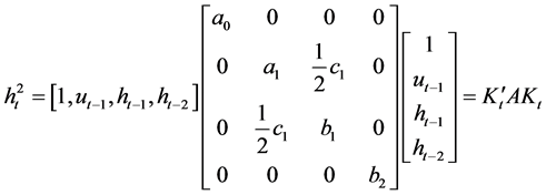 (2.4)
(2.4)
Proposition 1. A sufficient set of conditions for positivity of conditional variance ![]() is
is
 (2.5)
(2.5)
Proof. We note that  if and only if A is a positive definite matrix, and this implies that all eigenvalues of
  are strictly positive.
Set of these eigenvalues are:
 ■
■
2.2. Stationarity
We can rewrite the BL-GARCH (1, 2) as:


which is a random coefficient autoregressive model of second order [RCAR(2)].
We put: 
![]()

![]()
 and
and , we have
 (2.6)
(2.6)
 (2.7)
(2.7)
with ,
,  , and
, and  is backward operator. This implies that its eigenvalues are in the unit cercle.
So in order to the process be second order stationariry if and only if all eigenvalues are within unit cercle.
We can also rewrite the BL-GARCH (1, 2):
 (2.8)
(2.8)
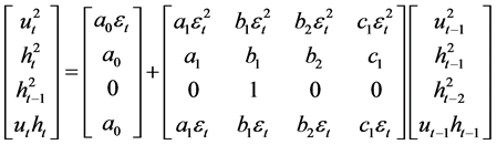 (2.9)
(2.9)
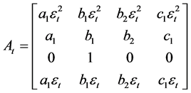
Remark 2. 1) ![]() is
is  matrix and
  in general case of BL-GARCH
  model.
2) Equation (2.8) is random coefficient VAR(1).
3)  is a Markov process.
Theorem 3. (strict stationarity)
In order to exist a strict stationary solution of Equation (2.8) it is necessary and sufficient that
 (2.10)
where , is the largest Lyapunov exponent of the model (2.8).
If this solution exists, then it is unique strictly stationary,non anticipative and ergodic.
Proof. See [11] . ■
Example 4. For the BL-GARCH (1, 2) we consider the matrix
for some values attributed to the coefficients ,
, ![]() ,
,  ,
, ![]() , we can simulate
, we can simulate  and
and  or
or .
.
Estimation of ![]() from
from ![]() simulations of size
simulations of size![]() .
.
This simulation does know us the region of stationarity of BL-GARCH (1, 2).
If , there is no stationary solution (strict or 2nd order), while there is a strictly stationary solution of an IGARCH model under general conditions.
2.3. Marginal Distribution
From (2.8) and by recursive, we have:

we put, for ,
,

we denote ![]() the Kronecker product and
the Kronecker product and ![]() matrix norm, then
matrix norm, then

using product matricies independence , because
  are
are , we have

If the spectral radius  of the matrix
 , then
  as
as , thus
![]() . So
. So  is sufficient condition for the exisrence of
 . For more details, it is recommended to refer to [11] .
Theorem 5. Suppose that  and
and , then for each
![]() ,
,  defined by (2.8) converge in
  and the process
  defined as the first component of
  is
is ![]() -order strictly stationary solution.
-order strictly stationary solution.
We make a simulation given some values of coefficients and a distribution of  in order to calculate
 ,
,  , and
, and .
.
3. The BL-GARCH Panel
We assumed that we have panel of asset returns, with ![]() observations and
observations and ![]() assets. The return on asset
assets. The return on asset ![]() at time
at time  is
is , where
  and
and , given by:
 (3.1)
(3.1)
where ,
,  and
and ,
, ![]() ,
,  with
with .
.
We consider  as a nuisance parameters, and
  as a vector of interest parameters. Using the covariance tracking, suggested by Engle and Mezrich [12] , we have:
 (3.2)
(3.2)
then we can use the method of moment to estimate the nuisance parameter. Assuming a stochastic independence over ![]() and
and , then the maximum likelihood estimator of
 ![]() is typically inconsistent for finite
is typically inconsistent for finite![]() , and
, and![]() . In order to overcome this problem and get a consistent estimator Engle, Shephard and Sheppard [13]
. In order to overcome this problem and get a consistent estimator Engle, Shephard and Sheppard [13]
allowed that ![]() to be large, and
to be large, and ![]() relates to
relates to ![]() and reduce the rate of convergence to
and reduce the rate of convergence to ![]() not
not noted in [13] , followed by the same study and consideration of Pakel, Shephard and Sheppard [9] .
3.1. Composite Maximum Likelihood
In this subsection we apply composite maximum likelihood method, that is widely used in time series in place of full likelihood when for example we want to reduce the computational complexity, or make inference about parameters of interest without making assumptions on the whole joint distribution of the data.
Given the data  where
where  and let
  be the conditional density for
 , we put
  and
and . Our estimation procedure focuses on two-step.
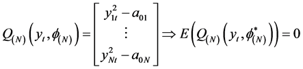
We begin by application of moment method to estimate nuisance parameters using (3.2), then we apply composite likelihood to estimate ![]() which is defined by:
which is defined by:
 (3.3)
(3.3)
In our situation we use the variation-free as Engle, Shephard and Sheppard [13] and Engle, Hendry and Richard [14] , then we obtain the composite maximum likelihood estimator by solving
 (3.4)
(3.4)
where  for each
 ![]() is obtained by solving
is obtained by solving

From (3.2) we have
 (3.5)
(3.5)
 (3.6)
(3.6)
where  is the true value of
  for each
![]() . Stacking (3.5) for
. Stacking (3.5) for , we have
 (3.7)
(3.7)
On the other hand, for the interest parameter![]() , we use composite likelihood, considering the following three typical distributions:
, we use composite likelihood, considering the following three typical distributions:
1) The score function for the normal density composite likelihood function is:
 (3.8)
(3.8)
2) The score function for the cauchy density composite likelihood function is:
 (3.9)
(3.9)
3) The score function for the student density composite likelihood function is:
 (3.10)
For  we put:
 (3.11)
where ![]() is a moment estimator.
is a moment estimator.
The sample moment conditions for each of (3.8), (3.9) and (3.10) are given by:
 (3.12)
We put:
then we imply that:

(3.6) and (3.11) are the first order condition for the maximisation problem of (3.4).
3.2. Asymptotic Behavior
In this subsection we attempt to obtain the asymptotic properties of composite likelihood estimator, based on a reasonable initial moment estimator for nuisance parameters. We show under which initial conditions to have a consistent estimator and asymptotic normality with the standard root—![]() convergence rate and
convergence rate and ![]() can potentially increase with
can potentially increase with![]() .
.
Engle, Shephard and Sheppard [13] have obtained consistency property and central limit theorem for  under some regularity conditions, and also Billy Wu, Qiwei Yao and Shiwu Zhu [15] . Through the following two fundamental theorems, we will show the consistency and central limit theorem for
  when
when ![]() while
while ![]() can potentially increase with
can potentially increase with![]() .
.
Theorem 6. We consider the following assumptions:
1) The condition (3.5) holds.
2) We assume that the parameters spaces are compacts.
3) Suppose that

4)  is continuously differentiable in
 .
.
5) Assume that the following sum satisfies a weak law large number as ![]()

6) Assume that

then there exists a solution of the likelihood Equation (3.11), for which 
Proof. See [13] . ■
Theorem 7. For any consistent solution of the likelihood Equation (3.11), we assume that:
1)  is once continuously differentiable.
2)  is an interior point of
 .
.
3) We put
4) We assume that  obeys a central limit theorem i.e.

where  is assumed that has diagonal elements definite positive.
5) That as , where
 ![]() is invertible.
is invertible.
then

Proof. The demonstration is well detailed in [13] . ■
4. Conclusion
Through this work, we have tried to study, in the first part the fundamental probabilistic properties of BLGARCH (1, 2), basing on studies of Abdou Kâ Diongue, D. Guégan and R. C. Wolff [4] and G. Storti & Vitale [1] , that have been made in this class of models. In the second part, we have studied the statistical inference, extended the model on panel data structure, and used one of efficient method well called composite likelihood that was introduced by Lindsay [6] . This method has good properties under some general regularity conditions as the consistency property and the asymptotic normality of estimators.
References
- Storti, G. and Vitale, C. (2003) BL-GARCH Models and Asymmetries in Volatility. Statistical Methods and Applications, 12, 19-40. http://dx.doi.org/10.1007/BF02511581
- Engle, R.F. (1982) Autoregressive Conditional Heteroscedasticity with Estimates of the Variance of United Kingdom Inflation. Econometrica, 50, 987-1007. http://dx.doi.org/10.2307/1912773
- Bollerslev, T. (1986) Generalized Autoregressive Conditional Heteroskedasticity. Journal of Econometrics, 31, 307-327. http://dx.doi.org/10.1016/0304-4076(86)90063-1
- Diongue, A.K., Guégan, D. and Wolff, R.C. (2009) BL-GARCH Models with Elliptical Distributed Innovations. Journal of Statistical Computation and Simulation, 80, 775-791. http://dx.doi.org/10.1080/00949650902773577
- Besag, J. (1974) Spatial Interaction and the Statistical Analysis of Latice Systems. Journal of the Royal Statistical Society: Series B, 36, 192-236.
- Lindsay, B. (1988) Composite Likelihood Methods. In: Prabhu, N.U., Ed., Statistical Inference from Stochastic Processes, American Mathematical Society, Providence, 221-239. http://dx.doi.org/10.1090/conm/080/999014
- Larribe, F. and Fearnhead, P. (2011) On Composite Likelihoods in Statistical Genetics. Statistica Sinica, 21, 43-69.
- Richard, A.D. and Chun, Y.Y. (2011) Comments on Pairwise Likelihood in Time Series Models. Statistica Sinica, 21, 255-277.
- Pakel, C., Shephard, N. and Sheppard, K. (2011) Nuisance Parameters, Composite Likelihoods and Panel of GARCH Models. Satistica Sinica, 21, 307-329.
- Monlenberghs, G. and Vervbeke, G. (2005) Models for Discrete Longitudinal Data. Springer, New York.
- Francq, C. and Zankoian, J.M. (2010) GARCH Models. Wiley, Hoboken. http://dx.doi.org/10.1002/9780470670057
- Engle, R.F. and Mezrich, J. (1996) GARCH for Groups. Risk, 9, 36-40.
- Engle, R.F., Shephard, N. and Sheppard, K. (2008) Fitting Vast Dimensional Time-Varying Covariance Models. Working Paper.
- Engle, R.F., Hendry, D.F. and Richard, J.F. (1983) Exogeneity. Econometrica, 51, 277-304.http://dx.doi.org/10.2307/1911990
- Wu, B., Yao, Q. and Zhu, S. (2013) Estimation in the Presence of Many Nuisance Parameters: Composite Likelihood and Plug-In Likelihood. Stochastic Processes and Their Applications, 123, 2877-2896.http://dx.doi.org/10.1016/j.spa.2013.03.017