Applied Mathematics
Vol.5 No.6(2014), Article ID:44607,21 pages DOI:10.4236/am.2014.56094
Anti-Robinson Structures for Analyzing Three-Way Two-Mode Proximity Data
Hans-Friedrich Köhn
Department of Psychology, University of Illinois, Urbana-Champaign, Champaign, USA
Email: hkoehn@cyrus.psych.uiuc.edu
Copyright © 2014 by author and Scientific Research Publishing Inc.
This work is licensed under the Creative Commons Attribution International License (CC BY).
http://creativecommons.org/licenses/by/4.0/


Received 27 December 2013; revised 27 January 2014; accepted 4 February 2014
ABSTRACT
Multiple discrete (non-spatial) and continuous (spatial) structures can be fitted to a proximity matrix to increase the information extracted about the relations among the row and column objects vis-à-vis a representation featuring only a single structure. However, using multiple discrete and continuous structures often leads to ambiguous results that make it difficult to determine the most faithful representation of the proximity matrix in question. We propose to resolve this dilemma by using a nonmetric analogue of spectral matrix decomposition, namely, the decomposition of the proximity matrix into a sum of equally-sized matrices, restricted only to display an order-constrained patterning, the anti-Robinson (AR) form. Each AR matrix captures a unique amount of the total variability of the original data. As our ultimate goal, we seek to extract a small number of matrices in AR form such that their sum allows for a parsimonious, but faithful reconstruction of the total variability among the original proximity entries. Subsequently, the AR matrices are treated as separate proximity matrices. Their specific patterning lends them immediately to the representation by a single (discrete non-spatial) ultrametric cluster dendrogram and a single (continuous spatial) unidimensional scale. Because both models refer to the same data base and involve the same number of parameters, estimated through least-squares, a direct comparison of their differential fit is legitimate. Thus, one can readily determine whether the amount of variability associated which each AR matrix is most faithfully represented by a discrete or a continuous structure, and which model provides in sum the most appropriate representation of the original proximity matrix. We propose an extension of the order-constrained anti-Robinson decomposition of square-symmetric proximity matrices to the analysis of individual differences of three-way data, with the third way representing individual data sources. An application to judgments of schematic face stimuli illustrates the method.
Keywords:Anti-Robinson Structure, Three-Way Data, Individual Differences, Ultrametric, Unidimensional Scale

1. Introduction
The structural representation of proximity data has always been an important topic in multivariate data analysis (see, for example, the monograph by Hubert, Arabie, and Meulman [1] ). The term proximity refers to any numerical measure of relation between the elements of two (possibly distinct) sets of objects. Proximities are usually collected into a matrix, with rows and columns representing the objects. Our concern here is only with square-symmetric proximity matrices, within the taxonomy of Carroll and Arabie [2] referred to as two-way one-mode proximity data; the way relates to the dimensionality of the matrix, and the mode to the number of sets of entities the ways correspond to. Proximities are assumed to be nonnegative, and WLOG, are henceforth interpreted as dissimilarities such that larger numerical values pertain to less similar pairs of objects.
The (casual) meaning of structural representation is captured by colloquialisms like “what goes with what” or “what is more or less than”. Mathematically, structural representation is defined here either in terms of a discrete non-spatial model or a continuous spatial model.
The former displays the relation between the row and column objects of the proximity matrix as a graph, with objects represented by nodes and dissimilarities fitted by edges of different length connecting the object nodes. The focus here is on the ultrametric tree structure, with objects arranged into nested categories—a display that is often referred to as a hierarchical cluster diagram. The continuous spatial model used here is the unidimensional scale: the interobject relations are translated into an ordering of objects along a line, with the dissimilarities fitted by the distances between objects. Both models are directly comparable for a given proximity matrix because they involve the same number of parameters estimable through least-squares minimization. Substantively, the two models address distinct perspectives on how objects are mentally represented.
Carroll [3] introduced the idea of fitting a proximity matrix by multiple continuous and discrete structures to increase the information extracted about the relations among the row and column objects vis-à-vis a representation featuring only a single structure (see also [1] -[6] ). However, it is often difficult to determine which particular set of multiple continuous and discrete structures provides the most faithful representation of a given proximity matrix. To illustrate, assume that for a given proximity matrix two (continuous) unidimensional scales provide superior overall fit as compared to a representation by two (discrete) ultrametric tree structures. At the same time, the first ultrametric tree structure attains substantially higher fit than the first unidimensional scale. We can only directly compare those two first structures. The second structures refer to different data bases. So, should we ultimately choose the discrete or the continuous representation?
We propose to resolve this ambiguity by using a nonmetric analogue of spectral matrix decomposition, namely, the additive decomposition of a proximity matrix into equally-sized matrices, constrained only to display a specific patterning among the cell entries called the anti-Robinson (AR) form. The AR form of a matrix is characterized by an ordering of its cells such that their entries are never-decreasing when moving away from the main diagonal [7] . As our ultimate goal, we seek to extract a small number of matrices in AR form such that their sum allows for a parsimonious, but faithful reconstruction of the total variability among the original proximity entries.
But why use the AR decomposition of the proximity matrix instead of the well-known spectral decomposition? A remarkable result in combinatorial data analysis states that fitting a unidimensional scale or an ultrametric tree structure to a square-symmetric proximity matrix generally produces matrices of distance and path length estimates that can be permuted into a perfect AR form [1] . Within this context, order-constrained AR matrix decomposition attains the status of a combinatorial data analytic meta-technique. Given their specific pattering, each extracted AR component relates immediately to the representation by a single unidimensional scale and a single ultrametric tree. As both models are directly comparable for each AR matrix, we can determine which structure provides a superior representation of the associated amount of variability—a feature not available when fitting multiple structures to a data matrix without order-constrained AR decomposition.
The extension of order-constrained AR matrix decomposition to accommodate three-way data for studying individual differences provides the analyst with an instrument to explore complex hypotheses concerning the appropriateness of continuous or discrete stimuli representations from an interindividual as well as an intraindividual perspective. We advocate an approach guided by a principle common in statistics as well as of immediate intuitive appeal, namely, to analyze individual variability within a deviation-from-the-mean framework. First, the individual proximity matrices are aggregated across sources into a single average matrix that is then fit by a small number of AR components (say, two or three). The identified AR decomposition serves as a frame of reference against which the individual proximity matrices are fit in a confirmatory manner, informing us how well the various individuals are represented by the reference decomposition. In addition, for each individual source, the obtained (comfirmatory) AR components themselves can be fit by unidimensional and ultrametric structures. Thus, we obtain (1) an interindividual assessment to what extent the various sources conform to the strucutral reference representation, and (2) an intraindividual comparison whether the distinct (confirmatory) AR matrix components are better represented in terms of a (continuous) unidimensional or (discrete) ultrametric model, with possible implications about the underlying individual cognitive representations of the stimuli.
The next section provides a summary of order-constrained AR matrix decomposition, while its generalization to accommodate three-way two-mode data is introduced in the third section. We conclude with an illustrative application of three-way order-constrained AR matrix decomposition for analyzing the structure of individual differences in judgments of schematic face stimuli.
2. Order-Constrained AR Matrix Decomposition
2.1. Definitions and Formal Concepts
Let  denote an
  square-symmetric proximity matrix, with
 ,
,  , and
, and . The rows and columns of
  represent a set of objects
 ; the
; the  have been characterized as pairwise dissimilarities of objects
 . Thus, in the following, we will consider solely the anti-Robinson (AR) form of proximity matrices, and their representation through sums of matrices of the according pattern. A square-symmetric matrix
  is said to have AR form if
 (1)
(1)
Verbally stated, moving away from the main diagonal of , within each row or column, the entries never decrease.
We seek a decomposition of  into the sum of matrices
 , with
  at most equall to
 , such that the least-squares loss function or
  -norm is minimized:

subject to the constraint of all  having AR form, where tr denotes the trace function, defined for an arbitrary
  matrix
  as
as .
.
The task of identifying an additive decomposition of  is addressed by fitting
  through subsequent residualizations of
 :
:  is fit to
 ,
,  to the residual matrix
 ,
,  to the residual matrix
 , and so on. However, the given proximity data matrix
  initially does not have AR form. Therefore, the rows and columns of
  need first to be re-arranged into a form that matches the desired AR pattern as closely as possible through identifying a suitable permutation
 , where
  denotes a permutation of the first
  integers. Similarly, the estimation of each subsequent AR component
  requires the preceding search for a permutation
 , producing a rearrangement of rows and columns of the involved residual matrices, optimally approximating the AR form. Hence, conceptually, generating an optimal AR decomposition of
  into
into  represents a two-fold (constrained) least-squares minimization problem; first, an operation to find a collection of permutations
 , for attempting to reorder the matrices into AR form, and second, an estimation step to numerically identify the desired AR components
  conforming to the order constraints as established through the respective permutations.
2.2. Optimal AR Decomposition: Algorithmic and Computational Details
The first task of searching for an optimal collection of permutations,  , represents an NP-hard combinatorial optimization problem, solvable by optimal solution strategies for object sets
  of small size, but calling for heuristic approaches for larger
 , yet with no guarantee of identifying the globally-optimal permutation. Note that for each component
  the number of distinct permutations equals
  because symmetry of
  precludes the necessity of considering reverse permutations. The search for the collection of optimal permutations,
  , can be carried out through a quadratic assignment (QA) heuristic. In general, solving the QA problem for two given
  matrices
  and
and , requires finding a permutation
  of the rows and columns of
  for fixed
  such that the sum of the products of corresponding cells is maximized:

[8] [9] . Define , with
 , which yields a perfect and equally spaced AR structure, and let
 , then

The fixed matrix  serves as the AR target: As the algorithm iteratively tries to maximize
 , the reordering mechanism by and by will match cells
  and
and  that maximally contribute to an increase of the QA-criterion. The search for a permutation
  that maximizes
  can be implemented through consecutive interchanges of single objects, or relocations of entire blocks of rows and columns of
 , until no improvement in
  can be found. Hence,
  represents an at least locally-optimal permutation, transforming
  to conform to the intended AR form as closely as possible. Consequently, the desired permutations in the collection,
  , are also at least locally-optimal. Alternative strategies for solving the QA problem include dynamic programming [10] and branch-and-bound algorithms [11] [12] .
The second optimization task of estimating the least-squares approximation  (in perfect AR form) to
  (denoting the permuted matrix), is carried out through iterative projection (IP) as proposed by Dykstra [13] [14] . In general, IP offers a computational strategy for solving constrained least-squares minimization problems. Let
  (with
(with ) denote a complete inner product space, also called a Hilbert space. The least-squares approximation to a vector
  is sought from a closed convex set
  in the form of a vector
  minimizing the least-squares criterion,
  , subject to linear constraints imposed on
  as defined by
 . Conceptually,
  can be found directly by projecting
  onto
onto ; in practice, however, this may pose extreme computational demands. Dykstra’s solution is as simple as it is elegant: based on the decomposition of the constraint set
 , the (presumably) difficult calculation of
  is broken down into the easier task of constructing a sequence
 , with
 , by way of iterative projections of
  onto the
  closed convex subsets of restrictions,
  , which, as was proven by Boyle and Dykstra [15] , converges to
 :
:

with  indicating the projection of
  onto
onto . The sequence
  is initialized by setting
 , followed by the projection of
  onto
onto , resulting in
 , in turn projected onto
 , yielding
  to be projected onto
 , and so on. The difference between consecutive projections
  and
and  is termed the increment, or residual. The algorithm concludes its first cycle of projections onto sets
 , with the projection of
  onto
onto  giving
 , the input vector for the second projection cycle through
 . However, from the second cycle on, each time
  are revisited in subsequent cycles, the increment from the previous cycle associated with that particular set has to be removed from the vector before actually proceeding with the projection.
Recall that, given the actual numerical entries in ,
,  indicates the best possible reordering of the
  rows and columns of
  into a form matching an AR pattern. Our goal is to estimate an
  least-squares approximation
  to
to , which has perfect AR form. Notice that the arrangement of the
  objects in
  has already been determined by
 . Thus, we can expand Equation (1) into a collection of
  sets of order constraints
 , which the desired numerical estimates
  have to satisfy. Each
  represents a single inequality of the form
  or
or . Formally, we need to find a perfect AR matrix
  minimizing the least-squares loss function,
 . Observe that the traceform of the loss function is equivalent to the earlier presented generic form
  if we vectorize
  and
and  into
into  and
and  by stacking the matrix columns into a vector, yielding the loss function
 , subject to the restriction
 . After initializing
  (recall that
  and
and ), the IP algorithm proceeds by checking for each adjacent pair of row and column objects whether the involved proximities conform to the respective constraints in
 . If at iteration
  a violation is encountered, the particular proximities are projected onto
  and replaced by their projections in iteration
  [13] . For example, if we observe
  the projections are given by:


Proceeding in this manner, IP cycles through  until convergence to
 .
.
Recall the objective to decompose  into a sum of identically-sized matrices in AR form,
 . The actual identification of the collection
  through successive residualizations of
  relies on engineering a complex interplay of the two optimization routines, QA and Dykstra’s IP. The algorithm is initialized by subjecting
  to a QA-based search for a permutation
  providing a rearrangement of the rows and columns of
 , matching the desired AR form as closely as possible, denoted by
 . Based on the order of row and column objects, as imposed by
 , the least-squares optimal AR matrix
  is fit to
  through the application of Dykstra’s IP procedure, with constraints
  derived from
  as defined by (1.1). By updating the target matrix,
  , through
 , we initiate a second QA search for a possibly superior permutation
  of
of  (of course,
  then remains fixed throughout the QA routine). The resulting
  will potentially even be closer to optimal AR patterning. Subsequently,
  is refit through IP. The algorithm cycles through QA and IP until convergence (i.e., updating
  by
by  does not result in any changes of
 ).
).
The residual matrix  is submitted to the search for the second AR component,
 . The algorithm switches back and forth between QA and IP, until
  and
and  have been identified, yielding the residual matrix
  to be forwarded to a third QA-IP search bearing
  and
and
 . The algorithm continues until a complete decomposition of
  has been attained, usually with
 . Evidently, the ultimate solution depends on the initial arrangement of rows and columns of
  (i.e., the particular order, in which
  is passed to the first QA search cycle); therefore, to reduce the risk of detecting a purely locally-optimal solution, a common nuisance to any heuristic procedure, multiple starts with random permutations are strongly recommended.
2.3. Low-AR-Rank Approximation to a Proximity Matrix
Spectral decomposition in linear algebra allows us to factor a given  proximity matrix into a sum of equally-sized matrices. Low-rank approximation refers to reconstructing the proximity matrix by a small number,
  , of those matrices. In an analogous manner, we can state our ultimate analytic objective so as to identify a smallest AR rank decomposition of
  such that
 , with
 . When only
  components in AR form are retrieved, the algorithm capitalizes on repetitively refitting the residuals of the different
 . Explicitly, assume that
  extracted AR components yield the residual matrix
 . In attempting to additionally improve the fit of the decomposition obtained, the residuals
  are added back to
 , succeeded by another run through the QA-IP fitting cycle, very likely detecting a more effective permutation
 , producing a revised
  to recalculate residuals
  that in turn are restored to the previously estimated
  component, which is then subjected to a new search for updating
 , and so on.
2.4. Fit Measure
The quality of a specific lower-AR-rank approximation to  is assessed by the variance-accounted-for (VAF) criterion. VAF is a normalization of the least-squares loss criterion by the sum of squared deviations of the proximities from their mean defined as
 (2)
(2)
where  denotes the mean of the off-diagonal entries in
 , and
, and  the fitted values of the
  AR component.
2.5. The Representation of AR Matrix Components
Each of the AR components  lends itself immediately to a more restricted representation, either in the form of a (continuous) unidimensional scale [16] -[18] of the elements in
  along a single axis, or through a (discrete) ultrametric tree diagram [19] .
For a specific AR component matrix , the unidimensional scale representation of its row/column objects can be constructed by estimating object coordinates
 ,
,  on the line minimizing the leastsquares loss function (by including an additive constant
 —see justification below):
 (3)
(3)
subject to the triangle (in)equality constraints on the coordinate values as implied by permutation  associated with
 :
:

An ultrametric tree structure can be characterized as a weighted acyclic connected graph with a natural root, defined as the node equidistant to all leaves or terminal nodes. The terminal nodes of an ultrametric tree represent a set of  objects
 . As a necessary and sufficient condition for a unique ultrametric tree representation, the weights along the paths connecting objects
 , typically with a distance interpretation and collected into an
  matrix
 , must satisfy the three-point condition or ultrametric inequality: for any distinct object triple
 ,
,  , and
, and , the largest two path length distances among
 ,
,  , and
, and  must be equal. Fitting an ultrametric structure
  to
to  also rests on minimizing a least-squares loss function:
 (4)
(4)
subject to the constraints as defined by the ultrametric inequality:

For a detailed technical description of how to construct a unidimensional scale or an ultrametric tree representation, the reader is encouraged to refer to the above references. The choice of these two models is justified by a remarkable result in combinatorial data analysis [1] [8] , which links them directly to the AR form of a square-symmetric proximity matrix. Specifically, the matrices of fitted interobject (unidimensional scale) distances and of estimated (ultrametric tree) path lengths can be permuted into perfect AR form. More to the point, optimal unidimensional scale and ultrametric tree structures induce the AR form of the matrices of fitted values. In other words, the AR form is a necessary condition for identifying these two more restricted models, as defined by the order constraints or the ultrametric inequality. We should re-emphasize that, for a given , both models involve the same number of parameters, estimable through least-squares. Thus, their VAF scores—
obtainable through normalizing the respective loss function by —are on an equal scale and directly comparable as to which structure provides a superior representation of
 . A brief technical note will be helpful to elaborate this claim. Recall that fitting the undimensional scale includes estimating an additive constant,
 . Employing a least-squares model without an additive constant would amount to fitting a regression model through the origin (in familiar generic notation:
 ), which—even though justifiable on theoretical grounds in certain instances—in general, has serious disadvantages. First, the residuals usually do not sum to zero; second, the sum of the squared residuals, SSE, might exceed the total sum of squares, SSTO, hence the coefficient of determination,
  , might turn out to be negative, thus becoming essentially meaningless. Lastly, using uncorrected
  as a remedy will avoid a negative
 , but
, but  will no longer be bounded between zero and one, creating another interpretation problem. Yet, by including an additive constant
  in the model,
  , we ensure that the obtained VAF fit score is equivalent to the (bounded)
  measure in regression. In the unidimensional scaling model, the additive constant is represented by
 . “Two interpretations exist for the role of the additive constant
 . We could consider
  to be fitted to the translated proximities
 , or alternatively,
  to be fitted to the original proximities
 , where the constant
  becomes part of the actual model” to be fitted to the untransformed proximities
  [1] . Once
  is established, constructing a unidimensional scale can be regarded as approximating the transformed proximities
  by the distances
 ; in other words, we are fitting a metric model (if the
  are subjected to an optimal monotone transformation, then the model represents nonmetric combinatorial unidimensional scaling). Fitting a least-squares intercept model implies the conjecture that the proximities have interval (and not ratio) scale properties.
One might object that the unidimensional scale model now has an additional parameter as compared to the ultrametric tree model. Notice, however, that in the special case of fitting a least-squares ultrametric structure, regression models with or without intercept are identical due to the particular structural side constraints imposed by the ultrametric inequality (thus, not necessitating the explicit inclusion of an additive constant, c):

Translation invariance does not hold for the unidimensional structure  to be fit to the
  as the triangle (in)equality constraints will be violated: let
  (and
(and ,
,  correspondingly), then

3. AR Matrix Decomposition for Three-Way Data
Three-way data, with the third way representing different data sources, such as subjects, experimental conditions, scenarios, or time points, represent a cube having multiple data matrices stacked as slices along the third dimension. Our concern here will be three-way two-mode data, so the slices will consist of square-symmetric proximity matrices of identical dimensions. By introducing the source index , the entire data cube is denoted by
 , and the layers of individual sources by
 .
.
The approach for modeling three-way data adopted in this paper is guided by a principle common in statistics as well as of immediate intuitive appeal, namely, to analyze individual variability within a deviation-from-themean framework: based on the individual proximity matrices aggregated across sources, denoted by , a best fitting reference AR decomposition is generated into
  average AR components, against which the individual data are fit. Concretely, assume that for
  the low AR rank approximation
  was chosen, with each component characterized by a unique ordering of
  as expressed by the associated permutations
  obtained from successive residualizations of
 . The componentwise object arrangements embodied in
  serve as a blueprint for (re)constructing the set of IP-constraints,
  , determining the specific AR form of
 , thereby providing a frame of reference for the AR decomposition of the
  individual proximity matrices in a confirmatory manner: as for each of the
  components the AR-optimal object order is fixed, the confirmatory fitting of the individual sources skips the QA step, and instead proceeds directly with estimating the
  source-specific AR components
  through IP, employing the
  sets of constraints
 .
.
The VAF criterion computed for each source separately serves as a fit index quantifying how closely the fitted proximities of the  of the individual AR decompositions reflect the properties of the reference structure:
 (5)
(5)
A source-specific unidimensional or ultrametric representation of the estimated AR components can be used for a direct evaluation of individuals’ fit against the reference structure, as well as for a more in-depth interand intra-subject analysis, be that by comparing the overall fit scores between sources or by specific fit of components  within a given source
 , to determine whether the continuous or discrete structure provides superior representation, with possible implications about the underlying individual cognitive processes.
4. Application: Judgments of Schematic Face Stimuli
A total of  graduate students in the Psychology department of the University of Illinois provided pairwise dissimilarity ratings of 12 schematic faces, displayed on a computer screen, on a nine-point scale. Not too different from previous work by Tversky and Krantz [20] , the twelve face stimuli were generated by completely crossing the three factors of “Facial Shape”, “Eyes”, and “Mouth” (see Figure 1).
The 22 individual matrices of dissimilarity ratings  were aggregated into a single matrix
  by first converting each individual’s ratings into z-scores (i.e., subtracting a person’s mean rating from each of his or her 66 dissimilarity ratings, and dividing these differences by his or her standard deviation), then averaging the z-scores across the 22 respondents for each pair of faces. Lastly, to eliminate negative numbers, and to put the aggregated dissimilarities back onto a scale similar to the original nine-point scale, the average z-score ratings were multiplied by 2, and a constant value of 4 was added.
The matrix  was subjected to a QA-IP-based search for an optimal AR decomposition with
  using multiple runs with initial random permutations of the input proximity matrix. For each decomposition into
  components, 10,000 random starts were used. The frequency distributions of the VAF scores obtained for each
  are reported in Table 1; the number of decimal places used may seem excessive, but is done here to make the distinct locally optimal solutions apparent.
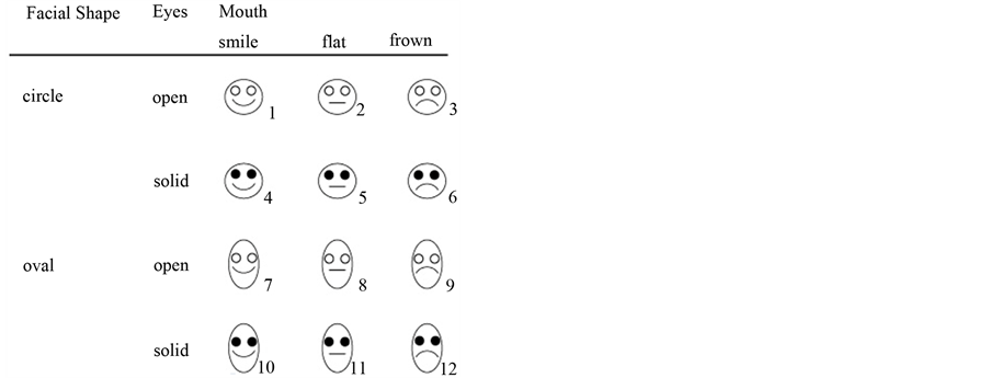
Figure 1. The construction of schematic face stimuli.

Table 1. Frequency distributions of the VAF scores as obtained from 10,000 random starts for .
.
Figure 2 presents the orders of facial stimuli as discovered for the  belonging to the AR decomposition of
  into
into  components with maximum VAF. Both the distribution results in Table 1 as well as the displays of the stimulus orderings in Figure 2 clearly suggest that the aggregated proximity matrix
  is of AR rank
 : first, the VAF increment for
  is minimal; second, while the order of stimuli associated with the first two components reveals an obvious pattern—
 : emotional appearance as captured by factor “Mouth”;
 : “circle” shaped versus “solid” eyes—the stimulus arrangements along the third and fourth AR components,
  and
and , lack such pattern. Lastly, across all four decompositions the first two AR components maintain a stable order of the stimuli (apart from a minimal inversion occurring on the second AR component concerning the two right-most faces), which does not hold for the third and fourth AR components. Thus, the biadditive solution with the largest VAF score (0.9593) was chosen as reference AR decomposition, against which the 22 individual rating matrices were fit.
The graphs of the unidimensional scale and ultrametric tree representation of the biadditive AR reference components  and
and  are shown in Figure 3. The interpretation is straightforward: the unidimensional scale constructed for
  orders the face stimuli along the continuum negative to positive expression of emotion, grouping them into three well-defined categories formed by the levels “frowning”, “flat”, and “smiling” of factor “Mouth” (the exact position of each face stimulus is at its left eye). The corresponding ultrametric tree structure of
  produces an almost perfectly balanced threefold segmentation of the face stimuli, also based on the primary criterion emotional appearance as expressed by the levels of factor “Mouth”. Notice that the three categories are not perceived as equally distinct; rather, “flat” and “smile” are merged, while “frown” is still set apart. Within each group, a secondary classification into faces according to “Facial Shape” can be observed, whereas “open” and “solid” circled eyes differentiate between stimuli at the tertiary level (note that this pattern is slightly violated by the “smile” segment). The unidimensional scale representing
  separates faces with “circle” shaped from “solid” eyes, with “oval” faced stimuli placed at the extreme scale poles—an arrangement of stimuli accurately reflected by the ultrametric tree structure. The latter also implies that “Facial Shape” and emotional appearance serve as subsequent descriptive features to group the stimuli. The tied triplet of “circle”
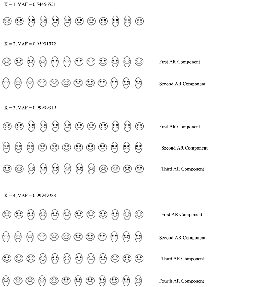
Figure 2. The orders of schematic face stimuli obtained for the various  components of the AR decompositions into K components with maximum VAF score.
shaped faces having “solid” eyes indicates a compromised fit of the ultrametric structure such as its imposition could only be accomplished by equating the respective stimulus distances. One might be tempted to conclude that the unidimensional scaling of the second AR component is degenerate because the twelve stimuli are lumped into four locations only. Upon closer inspection, however, this appears as an absolutely legitimate representation: the scale appropriately discriminates between “solid” and “circle” shaped eyes, while incorporating a secondary distinction based on facial shape. Thus, the retrieved scale accurately reflects a subset of constituting facial features ordering the stimuli in perfect accordance.
Each of the 22 individual source matrices,  , was then fitted against this biadditive AR reference structure —that is, the confirmatory biadditive AR decomposition of each of the individual proximity matrices was carried out, with the IP constraints derived directly from the object orderings associated with the two AR
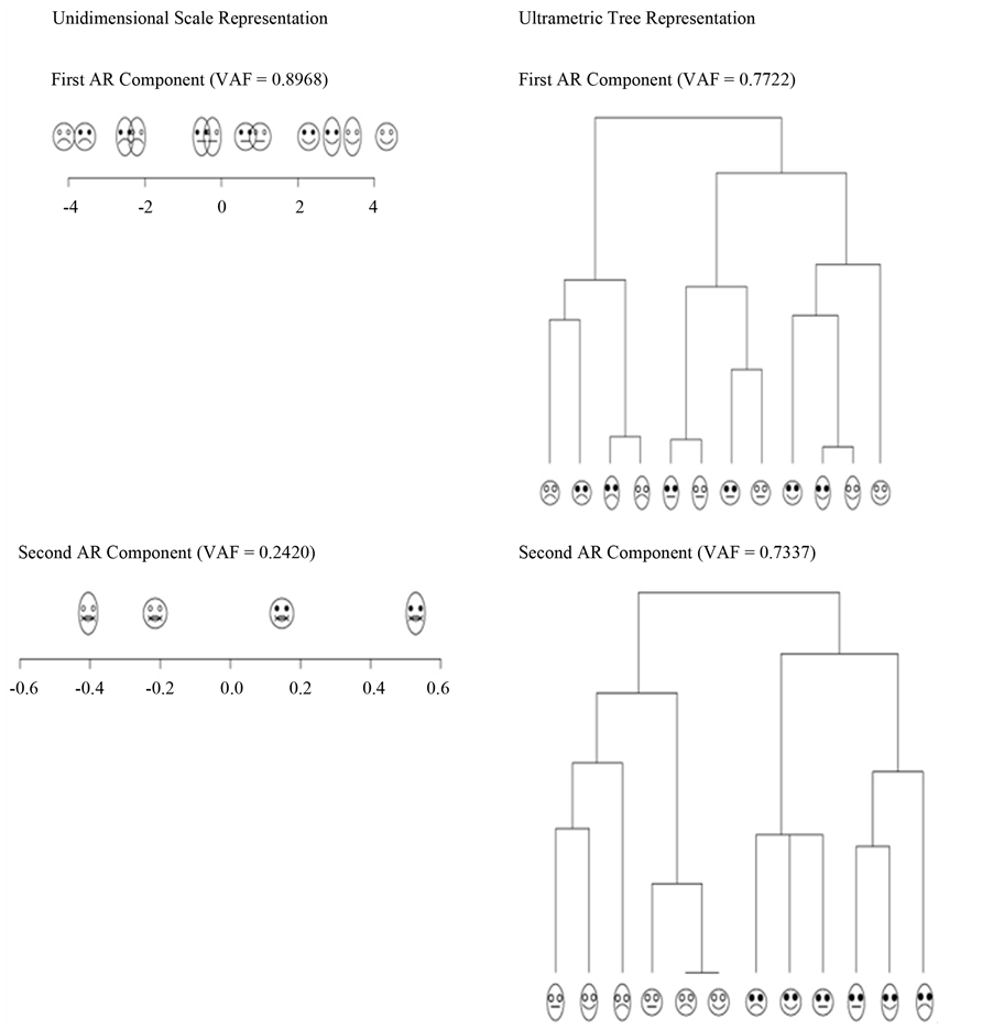
Figure 3. Biadditive reference AR decomposition of  (VAF = 0.959): unidimensional scale and ultrametric tree representations.
reference components. Table 2 presents the results for the 22 sources, sorted according to their VAF scores as defined by Equation (5), indicating how closely the various individuals actually match the biadditive reference AR structure. A variety of additional diagnostic measures is provided for assessing the differential contribution of the AR components  and
and . The VAF1 and VAF2 scores indicate how well the two AR components actually fit the corresponding residualizations of
 . They are defined in a manner similar to the overall or individual VAF measures in Equations (2) and (5), however, with minor modifications to adjust for the respective residualization; for example:

Table 2. Ranking of Individual VAF scores plus various fit measures quantifying the separate contributions of the two AR components  and
and .
.
where  denotes the mean of the residual matrix
 . Measures
  and
and  are obtained by refitting the final estimates of the AR components
  and
and  as sole predictors to the individual proximity matrices
  to assess their marginal variance contribution. The coefficients of partial determination
  and
and  quantify the marginal contribution of
  and
and  in reducing the total variation of
  when
when  or
or , respectively, has already been included in the model; for example:

with  denoting the sum of squared errors. Thus,
  indicates the sum of squared errors when
  serves as sole predictor, while
  represents the sums of squares due to error resulting when both AR components are in the model. Lastly, COV denotes the covariance of the two AR components defined by

In terms of the overall VAF score, subjects 11, 19, and 21 form the top three group, while the bottom three comprise subjects 1, 4, and 6, with the top and bottom three subjects marked by “ ”, and by “
 ”, respectively. For ease of legibility, all original fit scores were multiplied by 1000, thereby eliminating decimal points and leading zeros.
Table 3 reports the VAF scores obtained for the 22 sources when fitting unidimensional scales and ultrametric tree structures to the individual AR components  and
and . The VAF scores correspond to normalizations of the least-squares loss criteria in EquationS (3) and (4) by
 . For all sources, except subject 1, the unidimensional scaling of
  results in a much better fit than the corresponding ultrametric tree structure; however, for the second AR component, the ultrametric tree representation attains superior fit.
The most instructive course is to focus on the extremes and consider for further inspection only individuals who are exceptionally poorly or well represented: the top and bottom three subjects. For succinctness, from the top three group only the best fitting source, subject 11, was chosen for closer inspection. However, all three members of the bottom group, subjects 1, 4, and 6, were completely documented because they promised to provide deeper diagnostic insight into how sources with data of apparent ill-fit were handled by the AR
Table 3. Individual VAF scores for the unidimensional scale (US) and ultrametric tree (UT) representations of the two AR components  and
and .
.
decomposition. Figure 4 and Figure 5 present the unidimensional scales and ultrametric tree graphs fitted to the two individual AR components  and
and . For the ultrametric dendrograms the face stimuli have been arranged to match their order associated with the respective AR components; recall that for a fixed ultrametric structure there exist
  different ways of positioning the terminal object nodes of the tree diagram.
Not too surprising, the unidimensional scale as well as the non-spatial tree representations of  and
and  for subject 11 are almost identical to those of the reference structure, which by and large also applies to the unidimensional scales constructed for subjects 6 and 4. However, the findings for the latter two sources are put into perspective by the their ultrametric dendrograms: wildly dispersed branches, accompanied by several misallocations of stimuli, particularly for the representations of the second AR component, indicate an at best mediocre fit of the data from respondents 6 and 4 to the imposed AR structures. Such ambiguities do not pertain to subject 1, who is an obvious misfit: first, notice the equidistant alignment of stimuli along the unidimensional scale representing the first AR component, indicating a presumable lack of differentiation in the judgments of this subject. Moreover, inspecting the remaining three graphs corroborates the notion of the problematic nature of the data contributed by source 1 as the face stimuli appear to be arranged more or less in random order.
As an additional test of the conclusions from the confirmatory analysis, the individual data matrices of respondents 11, 6, 4 and 1 were reanalyzed through independent biadditive AR decompositions. Based on the logic that the confirmatory fitting could lead to a compromised structural representation of the individual data by imposing constraints inappropriate for a particular source, one might consider the obtained confirmatory configurations—in a transferred sense—as a lower bound representation. In other words, we would expect a well-fitting subject to profit from an independent analysis with the prospect of an only slightly better repressentation. For sources with poor fit, however, the independent analysis will either yield a substantial increase in fit because their idiosyncratic perspective, in disagreement with the majority of the sample, will no longer be distorted by an inadequate confirmatory reference frame, or these subjects will qualify as having provided simply inconsistent or random judgments not amenable to any improved data representation. Each of the four individual proximity matrices was was analyzed using 10,000 random starts. The solutions with the highest VAF score were chosen as final representations. The key diagnostics for subjects 11, 6, 4, and 1 are reported in Table 4. For all sources the overall VAF scores imply that their data are exhaustively approximated by an AR decomposition of rank .
.
The VAF scores for the unidimensional scale and ultrametric tree representations fit subsequently to the two AR components are presented in Table 5. As before, the unidimensional scale representations of the  attain much higher VAF values across all four sources than the ultrametric tree structures, while the latter provide superior representations of the second AR components
 .
.
For sources 11, 6, 4 and 1, graphs of the unidimensional scales and ultrametric tree structures for  and
and  are given in Figure 6 and Figure 7, respectively. The scale and dendrogram displays obtained for subject 11 afford an immediate interpretation: the arrangement of facial stimuli associated with the first AR component is dominated by the factor “Eyes”, with factors “Facial Shape” as secondary and “Mouth” as tertiary perceptual criteria; the ordering of faces identified with the second AR component is determined by the feature hierarchy “Mouth”, “Facial Shape” and “Eyes”. So, in comparison with the reference structure used for the confirmatory fitting, the independent analysis reveals that subject 11 employs the identical feature hierarchies, but reverses their association with the two AR components. For subject 6, the results are far less consistent. The independent analysis identifies “Mouth” as the primary factor, but in obvious disagreement with the first confirmatory AR component, the faces are no longer ordered along the meaningful emotional continuum “frown”—“flat”— “smile”. In addition, the secondary and tertiary criteria “Facial Shape” and “Eyes” are used inconsistently within these three groups—a finding also evidenced by the ultrametric tree. The branching pattern of the dendrogram indicates further inconsistencies in the grouping of stimuli as exemplified by the misclassifications of the two stimuli with “oval” face, “solid” eyes and “flat” mouth, or “circle” shaped face, “solid” eyes and “frowning” mouth line, respectively. The displays for the second AR component confirm these conclusions because both the unidimensional scale as well as the dendrogram are hardly interpretable and, rather resemble a non-systematic, ad hoc mix of factors “Facial Shape” and “Eyes”. Similar findings can be stated for subject 4: the scale as well as the tree representation of the first AR component appear to be determined by an inconsistent combination of factors “Eyes” and “Facial Shape”, while the arrangement of stimuli in the representations of the second AR component, seems to be governed by “Mouth”, but also in an inconsistent manner. In summarizing, remarkably and contrary to our expectations, respondents 6 and 4, do not emerge as subjects with a deviant, nevertheless

Figure 4. Confirmatory biadditive AR decomposition for selected sources: Unidimensional scale and ultrametric tree representations for the first AR component .
.
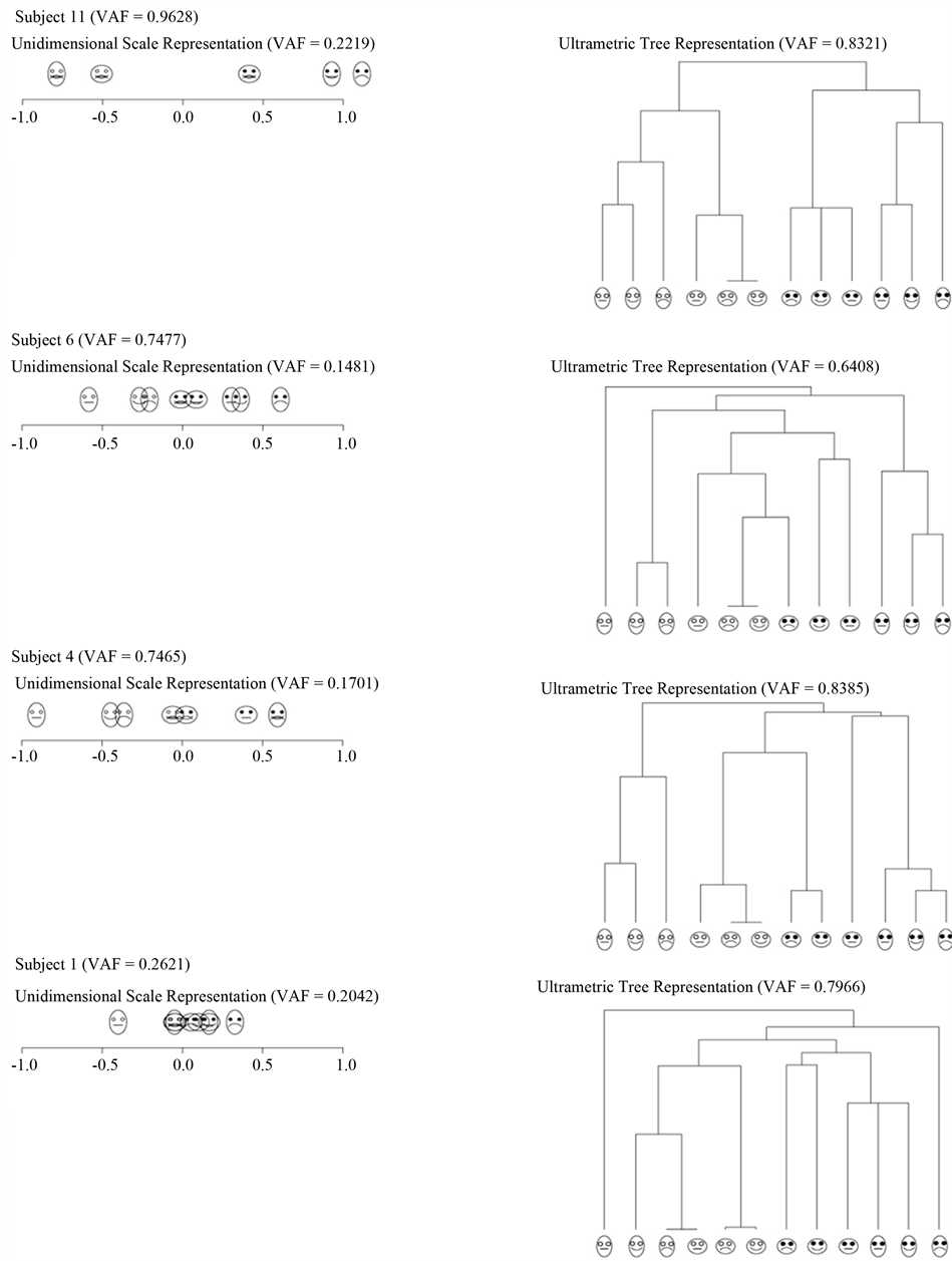
Figure 5. Confirmatory biadditive reference AR decomposition for selected sources: Unidimensional scale and ultrametric tree representations for the second AR component .
.
Table 4. Independent biadditive AR decomposition of selected sources: Individual VAF scores plus various fit measures quantifying the separate contributions of the two AR components  and
and .
.
Table 5. Individual VAF scores for the unidimensional scale (US) and ultrametric tree (UT) representations of the two AR components  and
and  from the independent analysis of selected sources.
well interpretable pattern of perceptual criteria, but as sources with profound inconsistencies in their judgments. The fuzzy results for source 1 allow for only an obvious explanation: the arrangement of the face stimuli reveals no discernable relation, implying that subject 1 merely contributed random responses.
5. Conclusions
In contrast to (traditional) calculus-based approaches, combinatorial data analysis attempts to construct optimal continuous spatial or discrete non-spatial object representations through identifying optimal object orderings, where “optimal” is operationalized within the context of a specific representation. For example, Defays [21] demonstrated that the task of finding a best-fitting unidimensional scale for given inter-object proximities can be solved solely by permuting the rows and columns of the data matrix such that a certain patterning among cell entries is satisfied. The desired numerical scale values can be immediately deduced from the reordered matrix. Similarly, for hierarchical clustering problems, in their more refined guise as searches for ultrametric or additive tree representations, optimal solutions are directly linked to particular permutations of the set of objects. Within this context, order-constrained AR matrix decomposition attains the status of a combinatorial data analytic meta technique, essentially pre-processing the observations: the total variability of a given proximity matrix is decomposed into a minimal number of separate AR components, each associated with a unique optimal object ordering related to distinct aspects of variation in the data. Based on the identified object permutations, the different AR components can be directly translated into continuous or discrete representations of the structural properties of the interobject relations. As the two models are fit through least-squares, they are directly comparable formally in terms of fit as well as interpretability—a feature not available when fitting multiple structures to a data matrix directly without initial decomposition. The extension of ordinal AR matrix decomposition to accommodate three-way data provides the analyst with an instrument to explore complex hypotheses concerning the appropriateness of continuous or discrete stimuli representations from an interindividual as well as intraindividual perspective.
From a substantive point of view, the results suggest that the set of schematic face stimuli is best represented by a combination of continuous spatial and discrete non-spatial structures: the first AR component, associated with factor “Mouth” and interpretable as emotional appearance, receives superior representation through a unidimensional scale, whereas the second AR component, reflecting a mix of “Facial Shape” and “Eyes”, is better represented by a discrete non-spatial structure—from hindsight not too surprising, given the specific manner in
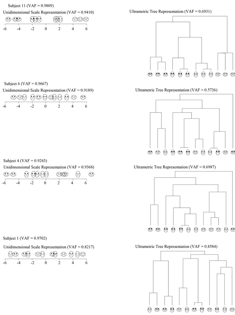
Figure 6. Independent biadditive AR decomposition for selected sources: Unidimensional scale and ultrametric tree representations for the first AR component .
.
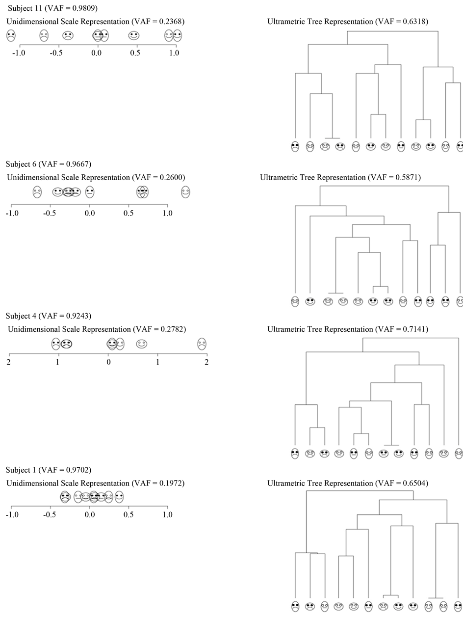
Figure 7. Independent biadditive AR decomposition for selected sources: Unidimensional scale and ultrametric tree representations for the second AR component .
.
which the stimuli were generated. The most remarkable finding concerns the independent analysis of subjects 6 and 4, who, despite numerically satisfactory fit scores, do not attain a more meaningful stimulus representation. Our initial hypothesis attributed their mediocre confirmatory fit to the biadditive AR reference structure as too restrictive for their distinctive perception. Contrary, the outcome of the independent analysis rather confirms the notion that these subjects simply entertained a weakly elaborated, inconsistent mix of criteria. The instantaneous question posed by these results—and definitely deserving future study—is whether an inconsistent, incomprehensible representation observed with a confirmatory AR decomposition provides sufficient diagnostic evidence to generally discredit the respective data set. More succinctly, is a questionable representation obtained from a confirmatory AR decomposition the incidental effect of an inappropriate structural frame of reference, or does it generally hint at data of poor quality, notwithstanding the context of a confirmatory or independent analysis? We may conjecture that the analysis of individual structural differences through AR decomposition is far less restrictive in its reliance on purely ordinal constraints, and, therefore, is not so susceptible to masking actual inconsistencies hidden in the data by the imposition of a more rigid (continuous) reference configuration.
As a final comment, given the extreme importance of the VAF criterion in selecting the AR reference decomposition as well as in assessing source-specific fit, conducting a large-scale simulation to study the behavior of the VAF measure deserves high priority. Of particular importance seems the question whether different object orders can result in identical VAF scores and to what extent different stimuli orders effect substantial alterations in VAF values.
References
- Hubert, L.J., Arabie, P. and Meulman, J. (2006) The Structural Representation of Proximity Matrices with MATLAB. SIAM, Philadelphia.
- Carroll, J.D. and Arabie, P. (1980) Multidimensional Scaling. Annual Review of Psychology, 31, 607-649. http://dx.doi.org/10.1146/annurev.ps.31.020180.003135
- Carroll, J.D. (1976) Spatial, Non-Spatial and Hybrid Models for Scaling. Psychometrika, 41, 439-463. http://dx.doi.org/10.1007/BF02296969
- Carroll, J.D. and Pruzansky, S. (1980) Discrete and Hybrid Scaling Models. In: Lantermann, E. and Feger, H., Eds., Similarity and Choice, Huber, Bern, 108-139.
- Carroll, J.D., Clark, L.A. and DeSarbo, W.S. (1984) The Representation of Three-Way Proximities Data by Single and Multiple Tree Structure Models. Journal of Classification, 1, 25-74. http://dx.doi.org/10.1007/BF01890116
- Hubert, L.J. and Arabie, P. (1995) Iterative Projection Strategies for the Least-Squares Fitting of Tree Structures to Proximity Data. British Journal of Mathematical and Statistical Psychology, 48, 281-317. http://dx.doi.org/10.1111/j.2044-8317.1995.tb01065.x
- Robinson, W.S. (1951) A Method for Chronologically Ordering Archaeological Deposits. American Antiquity, 19, 293- 301. http://dx.doi.org/10.2307/276978
- Hubert, L.J. and Arabie, P. (1994) The Analysis of Proximity Matrices through Sums of Matrices Having (Anti-)Robinson Forms. British Journal of Mathematical and Statistical Psychology, 47, 1-40. http://dx.doi.org/10.1111/j.2044-8317.1994.tb01023.x
- Rendl, F. (2002) The Quadratic Assignment Problem. In: Drezner, Z. and Hamacher, H.W., Eds., Facility Location, Springer, Berlin, 439-457. http://dx.doi.org/10.1007/978-3-642-56082-8_14
- Hubert, L.J., Arabie, P. and Meulman, J. (2001) Combinatorial Data Analysis: Optimization by Dynamic Programming. SIAM, Philadelphia. http://dx.doi.org/10.1137/1.9780898718553
- Brusco, M.J. (2002) A Branch-and-Bound Algorithm for Fitting Anti-Robinson Structures to Symmetric Dissimilarities Matrices. Psychometrika, 67, 459-471. http://dx.doi.org/10.1007/BF02294996
- Brusco, M.J. and Stahl, S. (2005) Branch-and-Bound Applications in Combinatorial Data Analysis. Springer, New York.
- Dykstra, R.L. (1983) An Algorithm for Restricted Least-Squares Regression. Journal of the American Statistical Association, 78, 837-842. http://dx.doi.org/10.1080/01621459.1983.10477029
- Deutsch, F. (2001) Best Approximation in Inner Product Spaces. Springer, New York. http://dx.doi.org/10.1007/978-1-4684-9298-9
- Boyle, J.P. and Dykstra, R.L. (1985) A Method for Finding Projections onto the Intersection of Convex Sets in Hilbert Spaces. In: Dykstra, R.L., Robertson, R. and Wright, F.T., Eds., Advances in Order Restricted Inference (Vol. 37), Lecture Notes in Statistics, Springer, Berlin, 28-47.
- Brusco, M.J. (2002) Integer Programming Methods for Seriation and Unidimensional Scaling of Proximity Matrices: A Review and Some Extensions. Journal of Classification, 19, 45-67. http://dx.doi.org/10.1007/s00357-001-0032-z
- Hubert, L.J. and Arabie, P. (1986) Unidimensional Scaling and Combinatorial Optimization. In: de Leeuw, J., Meulman, J., Heiser, W. and Critchley, F., Eds., Multidimensional Data Analysis, DSWO Press, Leiden, 181-196.
- Hubert, L.J. and Arabie, P. (1988) Relying on Necessary Conditions for Optimization: Unidimensional Scaling and Some Extensions. In: Bock, H.H., Ed., Classification and Related Methods of Data Analysis, Elsevier, Amsterdam, 463-472.
- Barthélemy, J.P. and Guénoche, A. (1991) Tree and Proximity Representations. Wiley, Chichester.
- Tversky, A. and Krantz, D. (1969) Similarity of Schematic Faces: A Test of Interdimensional Additivity. Perception and Psychophysics, 5, 124-128. http://dx.doi.org/10.3758/BF03210535
- Defays, D. (1978) A Short Note on a Method of Seriation. British Journal of Mathematical and Statistical Psychology, 31, 49-53. http://dx.doi.org/10.1111/j.2044-8317.1978.tb00571.x