ABSTRACT

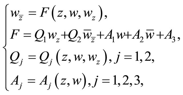
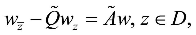
In this article, we discuss the approximate method of solving the Riemann-Hilbert boundary value problem for nonlinear uniformly elliptic complex equation of first order

(0.1)

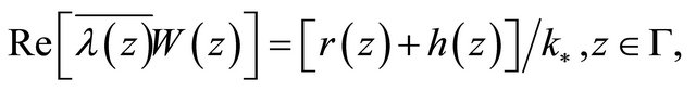
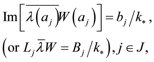
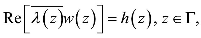
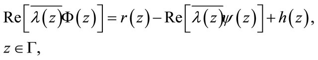
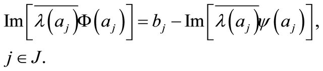
with the boundary conditions

(0.2)

in a multiply connected unbounded domain D, the above boundary value problem will be called Problem A. If the complex Equation (0.1) satisfies the conditions similar to Condition C of (1.1), and the boundary condition (0.2) satisfies the conditions similar to (1.5), then we can obtain approximate solutions of the boundary value problems (0.1) and (0.2). Moreover the error estimates of approximate solutions for the boundary value problem is also given. The boundary value problem possesses many applications in mechanics and physics etc., for instance from (5.114) and (5.115), Chapter VI, [1], we see that Problem A of (0.1) possesses the important application to the shell and elasticity.

1. Formulation of Elliptic Equations and Boundary Value Problem

Let be an -connected domain including the infinite point with the boundary inwhere. Without loss of generality, we assume that is a circular domain in, where the boundary consists of circles

,

and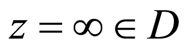. In this article, the notations are as the same in References [1-6]. We discuss the nonlinear uniformly elliptic complex equation of first order

(1.1)

which is the complex form of the real nonlinear elliptic system of first order equations

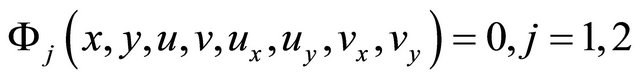(1.2)

under certain conditions (see [3]). Suppose that the complex Equation (1.1) satisfies the following conditions, namely Condition C: 1)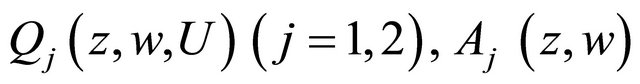

are measurable in for all continuous functions on and all measurable functions

and satisfy

(1.3)

where are non-negative constants.

2) The above functions are continuous in for almost every point and for

3) The complex Equation (1.1) satisfies the uniform ellipticity condition, i.e. for any, the following inequality in almost every point holds:

(1.4)

in which is a non-negative constant.

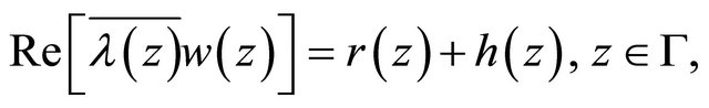
Problem A: The Riemann-Hilbert boundary value problem for the complex Equation (1.1) may be formulated as follows: Find a continuous solution of (1.1) on satisfying the boundary condition

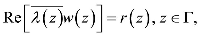(1.5)

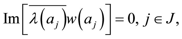
where and satisfy the conditions

(1.6)

in which are non-negative constants.

This boundary value problem for (1.1) with and will be called Problem The integer

is called the index of Problem and Problem

Due to when the index Problem may not be solvable, when the solution of Problem is not necessarily unique. Hence we put forward some well posednesses of Problem with modified boundary conditions.

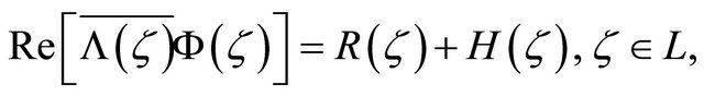
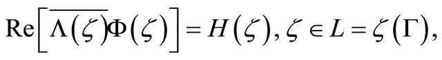
Problem B₁: Find a continuous solution of the complex Equation (1.1) in satisfying the boundary condition

(1.7)

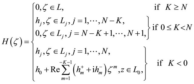
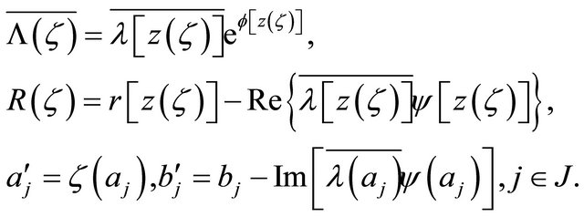
where

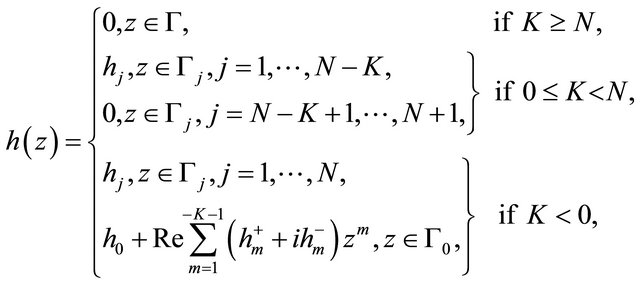
(1.8)

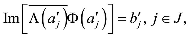
in which are unknown real constants to be determined appropriately. In addition, we may assume that the solution satisfies the following side conditions (point conditions)

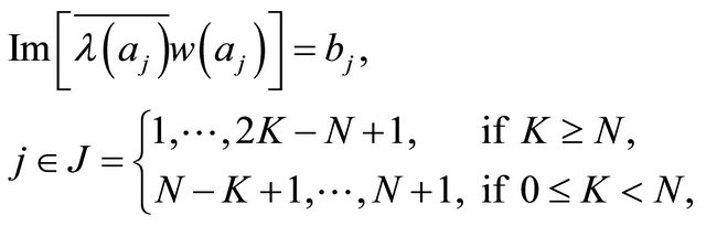(1.9)

where

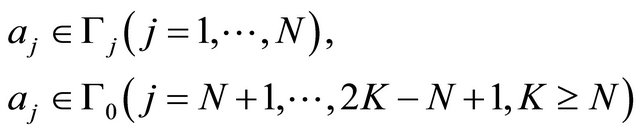
are distinct points, and are all real constants satisfying the conditions

(1.10)

herein is a nonnegative constant.

Now, we give the second well posed-ness of Problem.

Problem B₂: If the point condition (1.9) in Problem is replaced by the integral conditions

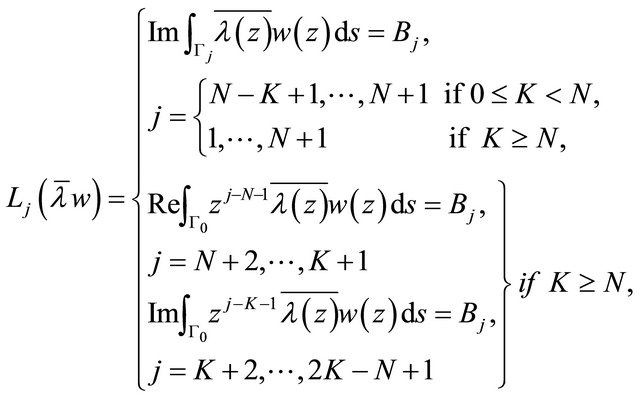
(1.11)

respectively, where are real constants satisfying the conditions

(1.12)

in which is a nonnegative real constant.

For convenience, we sometimes will subsume the integral conditions or the point conditions under boundary conditions.

2. A Priori Estimates of Solutions of Boundary Value Problem

First of all, we give a representation theorem of solutions for Problem and for Problem

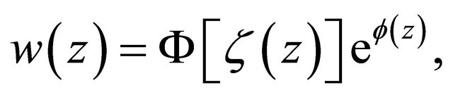
Theorem 2.1. Suppose that the complex Equation (1.1) satisfies Condition C, and is any solution of Problem (or Problem) for (1.1). Then is representable by

(2.1)

where is a homeomorphism on, which quasiconformally maps D onto an -connected circular domain G with boundary where the

are located in by

and is an analytic function in G, and its inverse function satisfy the estimates

(2.2)

(2.3)

(2.4)

in which are non-negative constants,

Proof. Similarly to Theorem 2.4, Chapter 2 in [3], we substitute the solution of Problem (or Problem) into the coefficients of the complex Equation (1.1) and consider the following system

(2.5)

(2.6)

(2.7)

By using the continuity method and the principle of contracting mappings, we can find the solutions

(2.8)

where

is a homeomorphism on is a univalent analytic function, which conformally maps onto an -connected circular domain, and is an analytic function in. We can verify that satisfy the estimates (2.2) and (2.3). Moreover noting that is a homeomorphic solution of the Beltrami complex Equation (2.7), which maps the circular domain onto the circular domain with the condition and in accordance with the result in Lemma 2.1, Chapter 2, [3], we see that the estimate (2.4) is true.

Now, we derive a priori estimates of solutions for Problem and for Problem for the complex Equation (1.1).

Theorem 2.2. Under the same conditions as in Theorem 2.1, any solution of Problem (or Problem) for (1.1) satisfies the estimates

(2.9)

(2.10)

where

are non-negative constants only dependent on and respectively.

Proof. On the basis of Theorem 2.1, the solution of Problem (or Problem) can be expressed the formula as in (2.1), hence the boundary value problem can be transformed into the boundary value problem (Problem) for analytic functions

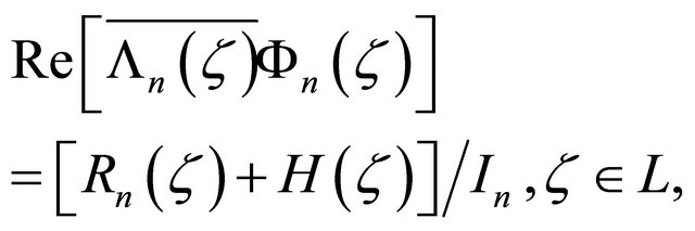
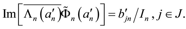
(2.11)

(2.12)

(2.13)

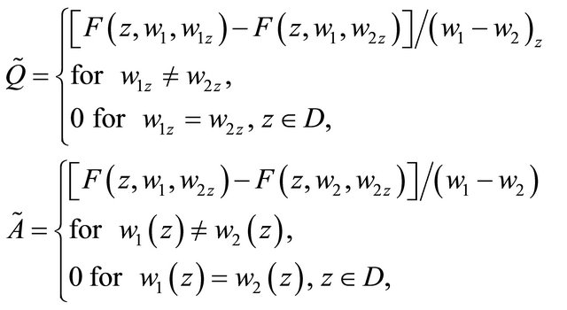
where

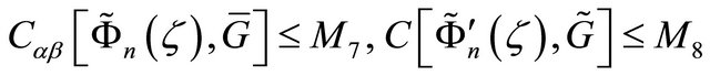
By (2.2)-(2.4), it can be seen that satisfy the conditions

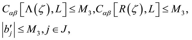(2.14)

where If we can prove that the solution of Problemsatisfies the estimate

(2.15)

in which

then from the representation (2.1) of the solution and the estimates (2.2)-(2.4) and (2.15), the estimates (2.9) and (2.10) can be derived.

It remains to prove that (2.15) holds. For this, we first verify the boundedness of, i.e.

(2.16)

Suppose that (2.16) is not true. Then there exist sequences of functions satisfying the same conditions as which uniformly converge to on L respectively. For the solution of the boundary value problem (Problem) corresponding to we have

as There is no harm in assuming that Obviously satisfies the boundary conditions

(2.17)

(2.18)

Applying the Schwarz formula, the Cauchy formula and the method of symmetric extension (see Theorem 1.4, Chapter 1, [3]), the estimates

(2.19)

can be obtained, where . Thus we can select a subsequence of which uniformly converge to an analytic function in, and satisfies the homogeneous boundary conditions

(2.20)

(2.21)

On the basis of the uniqueness theorem (see Theorem 2.4), we conclude that Howeverfrom it follows that there exists a point such that This contradiction proves that (2.16) holds. Afterwards using the method which leads from to (2.19), the estimate (2.15) can be derived.

Similarly, we can verify that any solution of Problem satisfies the estimates (2.9) and (2.10).

Theorem 2.3. Under the same conditions as in Theorem 2.1, any solution of Problem (or Problem) for (1.1) satisfies

(2.22)

where are as stated in Theorem 2.2,

Proof. If i.e. from Theorem 2.4, it follows that. If it is easy to see that satisfies the complex equation and boundary conditions

(2.23)

(2.24)

(2.25)

Noting that

and according to the proof of Theorem 2.2, we have

(2.26)

From the above estimates, it immediately follows that (2.22) holds.

Next, we prove the uniqueness of solutions of Problem and Problem for the complex Equation (1.1). For this, we need to add the following condition: For any continuous functions on and there is

(2.27)

where. When (1.1) is linear, (3.27) obviously holds.

Theorem 2.4. If Condition C and (2.27) hold, then the solution of Problem (or Problem) for (1.1) is unique.

Proof. Let be two solutions of Problem for (1.1). By Condition and (2.27), we see that is a solution of the following boundary value problem

(2.28)

(2.29)

(2.30)

where

and 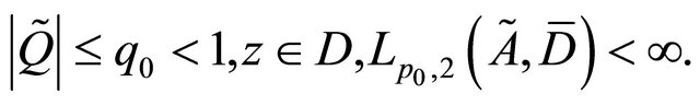According to the representation (2.1), we have

(2.31)

where are as stated in Theorem 2.1. It can be seen that the analytic function satisfies the boundary conditions of Problem

(2.32)

(2.33)

where are as stated in (2.11)-(2.13). In accordance with Theorem 2.2, it can be derived that Hence,

i.e.

3. The Continuity Method of Solving Boundary Value Problem

Next, we discuss the modified Riemann-Hilbert boundary value problems (Problem and Problem) for the nonlinear elliptic complex Equation (1.1) in the (N+1)-connected unbounded domain as stated in Section 1, here we use the Newton imbedding method of another form and give an error estimate, which is better than that as stated before. In the following, we only deal with Problem, because by using the same method, Problem can be discussed.

Theorem 3.1. Suppose that the nonlinear elliptic Equation (1.1) satisfies Condition C and (1.6), (1.10), on. Then Problem for (1.1) has a solution

Proof We introduce the nonlinear elliptic complex equation with the parameter:

(3.1)

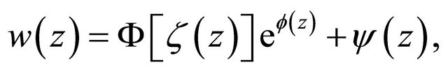
where is any measurable function in and When, it is not difficult to see that there exists a unique solution of Problem for the complex Equation (3.1), which possesses the form

(3.2)

where is an analytic function in and satisfies the boundary conditions

(3.3)

(3.4)

From Theorem Theorem 2.2, We see that

Suppose that when, Problem for the complex Equation (1.18) has a unique solution, we shall prove that there exists a neighborhood of

so that for every

and any function Problem for (1.18) is solvable. In fact, the complex Equation (3.2) can be written in the form

(3.5)

We arbitrarily select a function

in particular

on. Let be replaced into the position of in the right hand side of (1.22). By Condition, it is obvious that

Noting the (3.5) has a solution Applying the successive iteration, we can find out a sequence of functions: which satisfy the complex equations

(3.6)

The difference of the above equations for and n is as follows:

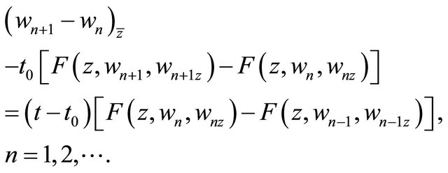(3.7)

From Condition, on, it can be seen that

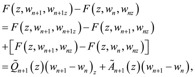
and

Moreover, satisfies the homogeneous boundary conditions

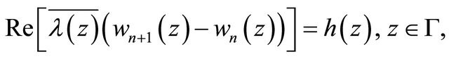(3.8)

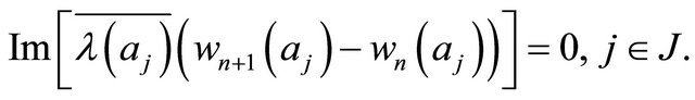(3.9)

On the basis of Theorem 2.3, we have

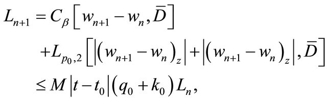(3.10)

where is as stated in (2.22). Provided is small enough, so that

it can be obtained that

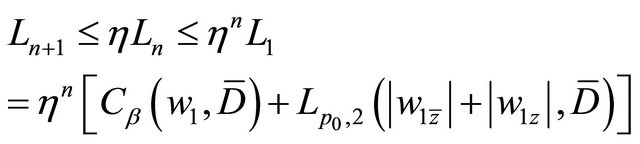(3.11)

for every Thus

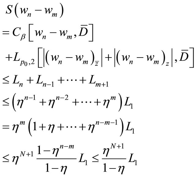(3.12)

for where is a positive integer. This shows that as Following the completeness of the Banach space

there is a function such that when

By Condition and (1.6), (1.10), from the above formula it follows that is a solution of Problem for (3.5), i.e. (3.1) for. It is easy to see that the positive constant is independent of. Hence from Problem for the complex Equation (3.1) with is solvable, we can derive that when, Problem for (3.1) are solvable, especially Problem for (3.2) with and, namely Problem for (1.1) has a unique solution.

4. Error Estimates of Approximate Solutions for Boundary Value Problem

In this section, we shall introduce an error estimate of the above approximate solutions of the boundary value problem and can give the following error estimate of the approximate solutions.

Theorem 4.1 Let be a solution of Problem for the complex Equation (1.1) satisfying Condition and (1.6), (1.10) on, and be its approximation as stated in the proof of Theorem 2.2 with Then we have the following error estimate

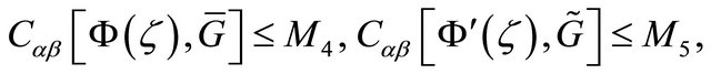
(4.1)

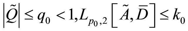
where

and are constants in (1.3), (1.6) and (1.10).

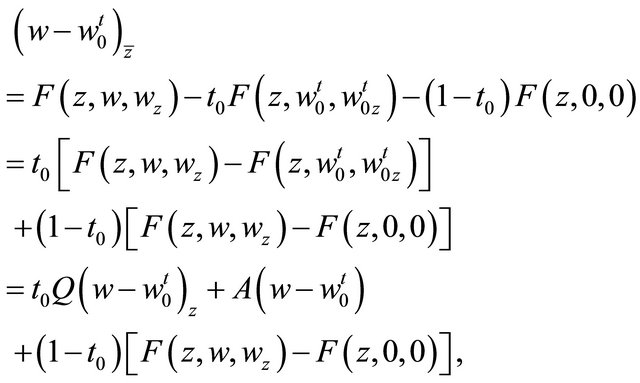
Proof From (1.1) and (2.23) with , we have

(4.2)

It is clear that satisfies the homogeneous boundary conditions

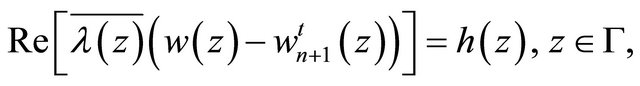(4.3)

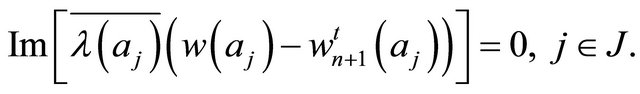(4.4)

Noting that

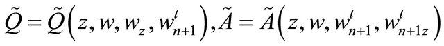satisfy

, and

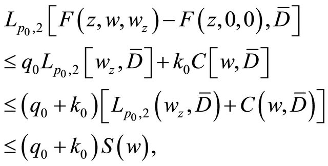
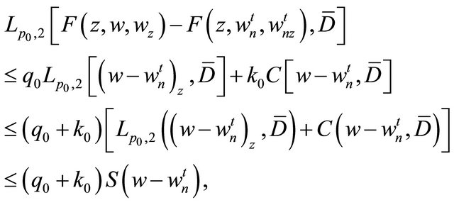
and according to Theorem 2.2, it can be concluded

(4.5)

where and

(4.6)

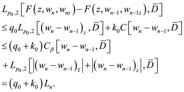
where are non-negative constants as stated in (1.3), (1.6) and (1.10). From (4.5) and (4.6), it follows

where and we choose that is the solution of Problem for (2.22) with and Due to is a solution of Problem for the complex equation

(4.7)

hence

(4.8)

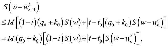
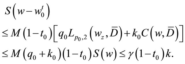
Finally, we obtain

(4.9)

this shows that (4.1) holds. If the positive constant is small enough, so that when is sufficiently large and is close to 1, then the right hand side becomes small.

REFERENCES

- I. N. Vekua, “Generalized Analytic Functions,” Pergamon, Oxford, 1962.
- G. C. Wen, “Linear and Nonlinear Elliptic Complex Equations,” Shanghai Scientific and Technical Publishers, Shanghai, 1986.
- G. C. Wen and H. Begehr, “Boundary Value Problems for Elliptic Equations and Systems,” Longman Scientific and Technical Company, Harlow, 1990.
- G. C. Wen, “Approximate Methods and Numerical Analysis for Elliptic Complex Equations,” Gordon and Breach, Amsterdam, 1999.
- G. C. Wen, D. C. Chen and Z. L. Xu, “Nonlinear Complex Analysis and Its Applications,” Mathematics Monograph Series 12, Science Press, Beijing, 2008.
- G. C. Wen, “Recent Progress in Theory and Applications of Modern Complex Analysis,” Science Press, Beijing, 2010.