Applied Mathematics
Vol.3 No.12(2012), Article ID:25467,5 pages DOI:10.4236/am.2012.312265
Numerical Solution of Functional Integral and Integro-Differential Equations by Using B-Splines
1Department of Mathematics, Karaj Branch, Islamic Azad University, Karaj, Iran
2Faculty of Education, Universiti Teknologi Malaysia, Johor, Malaysia
Email: *derili@kiau.ac.ir, hmohamadikia@yahoo.com
Received September 20, 2012; revised October 20, 2012; accepted October 28, 2012
Keywords: Lagrange Interpolation; B-Spline Functions; Functional Integral Equation; Functional Integro-Differential Equation; Functional Differential Equations
ABSTRACT
This paper describes an approximating solution, based on Lagrange interpolation and spline functions, to treat functional integral equations of Fredholm type and Volterra type. This method extended to functional integral and integro-differential equations. For showing efficiency of the method we give some numerical examples.
1. Introduction
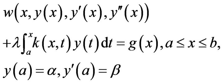
In recent years there has been a growing interest in the numerical treatment of the functional differential equations,
 (1)
(1)
which is said to be of retarded type if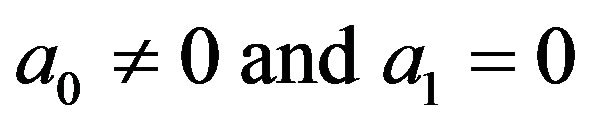 . It is said to be natural type
 . If
. If 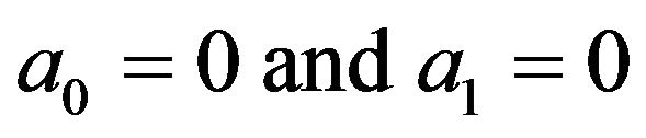 it is said to be advanced type. For more general functional equations see Arndt [1], In further details many authors such as, El-Gendi [2], Zennaro [3], Fox, et al. [4].
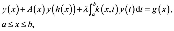
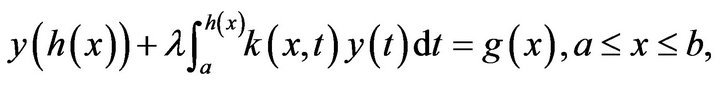
Rashed introduced new interpolation method for functional integral equations and functional integro-differential equations [5]. In this paper we approximate the numerical solution  of the following functional integral equations and integro-differential equations:
 (2)
(2)
 (3)
(3)
 (4)
(4)
 (5)
(5)
 (6)
(6)
where
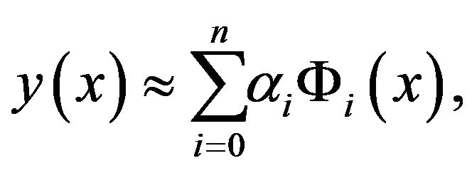
For this approximation we first interpolate 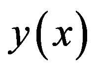 with following interpolation formula:
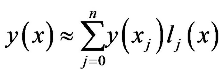 (7)
(7)
where
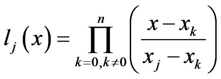 (8)
(8)
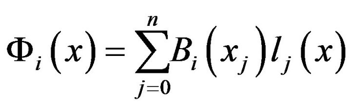
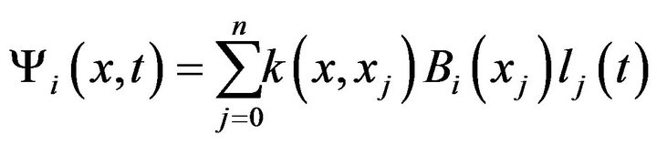
and
 (9)
(9)
where
 (10)
(10)
where  is a well known function.
Then for computing  we use B-Spline approximation that we present its details in the next section [6-9]. In the third section we give our method for functional integral equations. Also the fourth section is devoted to numerical solution of integro-differential equations. Of course for computing integrals both in the third and the fourth section we used Clenshaw-Curtis rule [10,11]. Finally in the latest section we give some applications of both functional integral equations and integro differential equations with numerical solutions. In addition, we compared our results with Rashed method [5,12]. We present some additional conclusions in Section 6.
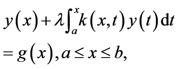
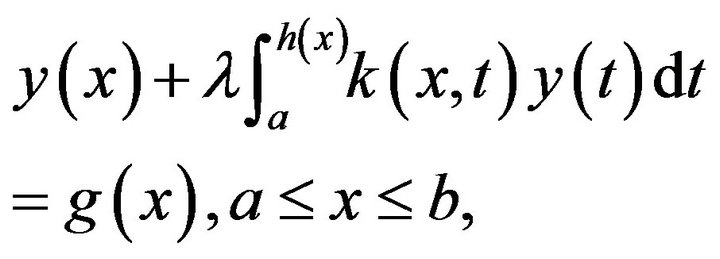
2. Functional Linear Integral Equations of the Second Kind
In this paper we use spline function with Lagrange interpolation to compute the numerical solution  of functional linear integral equations of the second kind:
 (11)
(11)
 (12)
(12)
 (13)
(13)
 (14)
(14)
In fact, We seek to find an approximation to ![]() which satisfies some interpolation property or variational principle.
which satisfies some interpolation property or variational principle.
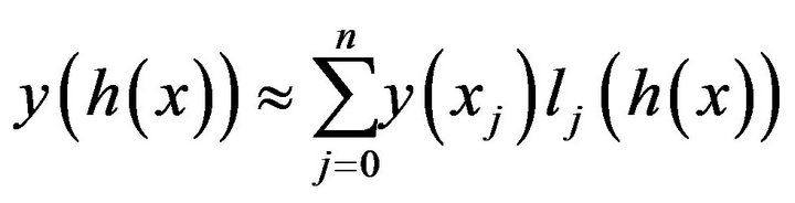
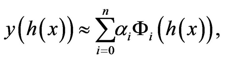
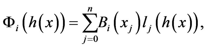
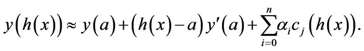
In this functional integral Equations (2)-(5), we may use Lagrange interpolation of  by
by
 (15)
(15)
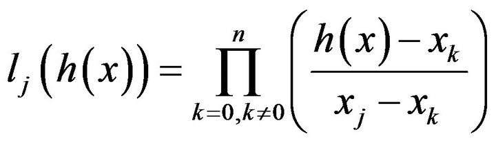
where
 (16)
(16)
and
 (17)
(17)
and also
 (18)
(18)
where
 (19)
(19)
and
 (20)
(20)
where  is well known function. Also
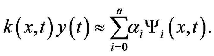 (21)
(21)
 (22)
(22)
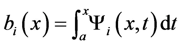
The integral part of each functional Equations (2)-(5) is given as follows: Integrating (1) w.r.t  from
from ![]() to
to ![]()
 (23)
(23)
 (24)
(24)
Integrating (10) w.r.t  from
from ![]() to
to 
 (25)
(25)
 (26)
(26)
Integrating (10) w.r.t  from
from ![]() to
to 
 (27)
(27)
where
 (28)
(28)
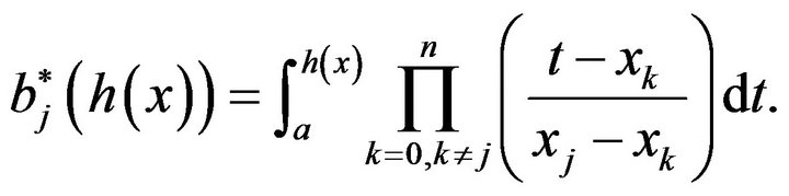 (29)
(29)
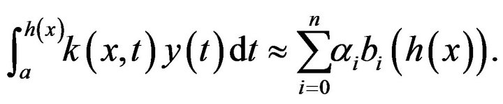
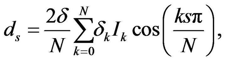
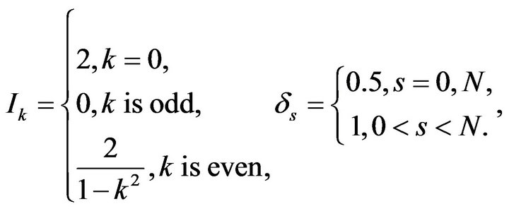
The integral in the relation (21) is approximated as:
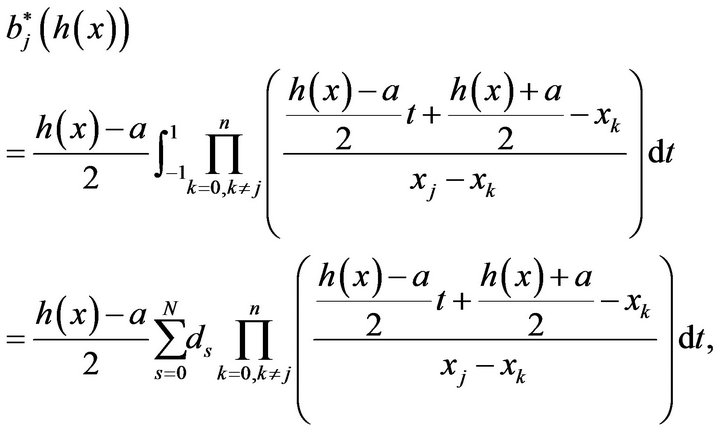 (30)
(30)
where
Finally, the functional integral equation is approximated by system of ![]() linear equations. Also, the method is extended to treat the functional equations of advanced type (
linear equations. Also, the method is extended to treat the functional equations of advanced type ( in
in  or
or )
)
 (31)
(31)
The last equation may not has analytically solution.
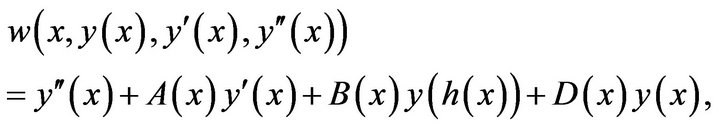
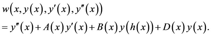
3. Functional Linear Integro-Differential Equations of the Second Kind
Consider the functional integro-differential equation of the second equation
 (32)
(32)
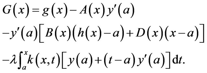
where
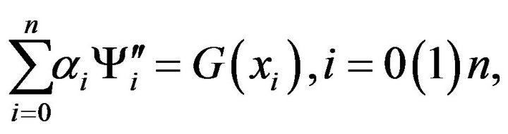
With using Lagrange interpolation, the second derivative 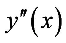 is given by
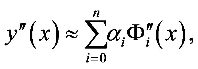 (33)
(33)
where
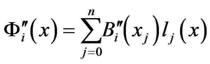 (34)
(34)
Integrating (35) w.r.t ![]() from
from ![]() to
to ![]()
 (35)
(35)
Integrating (37) w.r.t ![]() from
from ![]() to
to ![]()
 (36)
(36)
The integral is computed as (31). Also, integrating (36) w.r.t ![]() from
from ![]() to
to 
 (37)
(37)
Substitution from (37) to (40) into (34) lead to system of ![]() linear equations
linear equations
where

 (38)
(38)
and
 (39)
(39)
The integrals in (40) and (41) may be computed by Clenshaw-Curtis rule. It is obviously that the method may be extended to functional linear differential equations of the second order if  in (34).
4. Numerical Examples
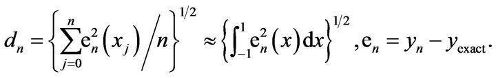
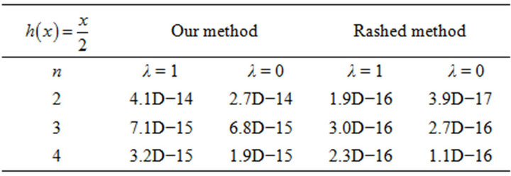
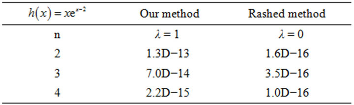
We compared our results with Rashed results [5]. We consider here the following examples on the functional integral equation, integro-differential and differential equations for comparison. The computed errors  in these tables are defined to be
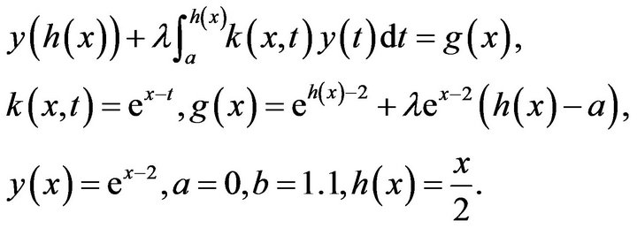
Example 1. Volterra integral equation of the second kind
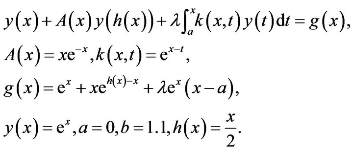

Example 2. Fredholm integral equation of the second kind

Example 3. Volterra integral equation of the second kind

Example 4. Volterra integral equation of the second kind

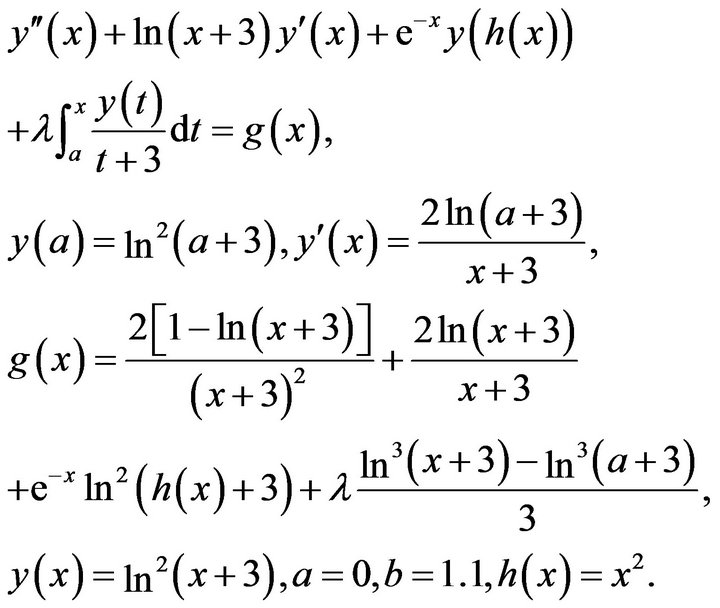
Example 5. Volterra integro-differential equation of the second kind
5. Conclusions
1) The method give the approximate solution at the points

2) The method can be extended to the functional differential equation
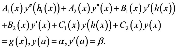
3) The method may be used to treat boundary functional differential or integro-differential equations.

4) The small errors obtained shows that the method indeed successfully approximate the solution of problem.
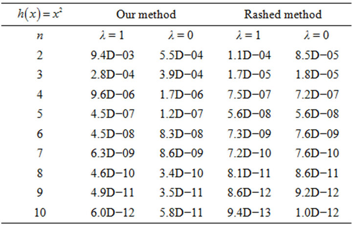
Remark 1 The spline piecewise functions are very essential tools in approximation Theory. Then for this we applied B-Splines for approximation of unknown answer in integro-differential equations. From Tables, We see that for mesh points with , we have small errors. Therefore the mentioned results for
  have high quality and application of B-Splines is acceptable (of course for getting convenient answer we must had
 ).
).
REFERENCES
- H. Arndt, “Numerical Solution of Retarded Initial Value Problems: Local and Global Error and Step-Size Control,” Numerische Mathematik, Vol. 43, No. 3, 1984, pp. 343-360. doi:10.1007/BF01390178
- S. E. El-Gendi, “Chebyshev Solution of a Class of Functional Equations,” Computer Society of India, Vol. 8, 1971, pp. 271-307.
- M. Zennaro, “Natural Continuous Extension of RungeKutta Methods,” Mathematics of Computation, Vol. 46, No. 173, 1986, pp. 119-133. doi:10.1090/S0025-5718-1986-0815835-1
- L. Fox, D. F. Mayers, J. R. Ockendon and A. B. Taylor, “Ona Functional Differential Equation,” Journal of the Institute of Mathematics and Its Applications, Vol. 8, No. 3, 1971, pp. 271-307. doi:10.1093/imamat/8.3.271
- M. T. Rashed, “Numerical Solution of Functional Differential, Integral and Integro-Differential Equations,” Applied Mathematics and Computation, Vol. 156, No. 2, 2004, pp. 485-492. doi:10.1016/j.amc.2003.08.021
- K. Maleknejad and S. Rahbar, “Numerical Solution of Fredholm Integral Equations of the Second Kind by Using B-Spline Functions,” International Journal of Engineering Science, Vol. 11, No. 5, 2000, pp. 9-17.
- J. Stoer and R. Bulirsch, “Introduction to the Numerical Analysis,” Springer-Verlag, New York, 2002.
- L. L. Schumaker, “Spline Functions: Basic Theory,” John Wiley, New York, 1981.
- C. T. H. Baker, “The Numerical Solution of Integral Equations,” Clarendon Press, Oxford, 1969.
- K. Maleknejad and H. Derili, “Numerical Solution of Integral Equations by Using Combination of Spline-Collocation Method and Lagrange Interpolation,” Applied Mathematics and Computation, Vol. 175, No. 2, 2006, pp. 1235-1244.
- L. M. Delves and J. L. Mohammed, “Computational Methods for Integral Equations,” Cambridge University Press, Cambridge, 1985. doi:10.1017/CBO9780511569609
- M. T. Rashed, “An Expansion Method to Treat Integral Equations,” Applied Mathematics and Computation, Vol. 135, No. 2-3, 2003, pp. 73-79. doi:10.1016/S0096-3003(02)00347-8
NOTES
*Corresponding author.