International Journal of Geosciences
Vol. 3 No. 4 (2012) , Article ID: 22928 , 9 pages DOI:10.4236/ijg.2012.34080
Stochastic Modelling and Geological Aspects of a Gold Mineralisation
1Department of Statistics, Sri Venkateswara University, Tirupati, India
2Guru Nanak Institute of P. G. Studies, Formerly Scientist-G, NGRI (CSIR), Hyderabad, India
Email: ganimsc2007@gmail.com, drddsarma@gmail.com, putharsr@yahoo.co.in
Received May 22, 2012; revised June 24, 2012; accepted July 2, 2012
Keywords: Estimation; Geometry; Gold mineralization; Stochastic Process; Regionalized Variables; Strike Reef
ABSTRACT
Gold mineralisation is the result of physico-chemical and thermal processes of the earth’s interior. We may view a geological process of gold mineralization as a stochastic process Z(x): xÎD, where D may be considered as a mineral deposit. In the case of gold mineralization, samples drawn at regular intervals may be considered as following a discrete stochastic process. The point of interest is one of realistic estimation of mineral value property as computations based on classical methods leading to erroneous results. Modern methods based on stochastic modelling treating the process as an 1) Auto-regressive (AR); 2) Moving-average (MA) or a combination of these two viz.; 3) ARMA of appropriate order k may lead to more realistic results. Yet another class of methods which consider the geometry of samples in termed as theory of Regionalised Variables. This paper analyses these classes of methods and illustrates a case study of a gold mineralization related to Strike Reef (Footwall branch) of Hutti gold mines.
1. Introduction
Mineralisation formation by geological process may be considered as a discrete stochastic process . In the case of gold mineralisation process, samples drawn at regular interval may be considered as a discrete stochastic process. It is of utmost interest to estimate the mineral value properties and say grade/accumulation. Towards this end, time series analysis/stochastic modelling may be of utmost importance. Sarma [1-3] discussed application of time series special reference to gold and copper mineralization. Sarma and Koch [4] discussed the application of statistical technique to Uranium exploration problem. Sahu [5,6] carried out statistical modelling and time series analysis applied to mineral deposit modelling and evaluation.
This paper deals with stochastic and geo-statistical aspects of Strike Reef (Footwall branch) of Hutti gold mines emphasising auto-correlation function and semivariogram as basic tools for drawing inferences and interpretation. The Mines at Hutti are shallow in depth, usually not exceeding 1000 m. A problem here is to obtain realistic estimates of gold value properties. Proper estimation of gold content leads to an adequate estimation of grade content and ore reserves.
2. Data
The data for the present study constitute chip samples taken from the mineralised rock of Strike Reef (Footwall branch) of Hutti gold mines. Chip samples of mineralised rock weighing about 1 - 2 kg are collected on the width of the reef at each sampling point and assayed. The distance between one sampling point and other which is called sampling interval is 1 m. The analyzed gold content per tonne of ore and the width of reef at that sampling point are recorded. Thus, the unit of measurement is g/t of ore for grade and meter-grade (mg) for accumulation. Accumulation at any sampling point is the product of width of the reef in m or cm and the grade at that point. The sample sizes considered for analysis for each of the levels of Strike Reef are given in Table 1.
The data comprising grade and accumulation values of the above mentioned lode, which extends up to a depth of 600 m were first analyzed to understand the nature of the distribution. Graphical plot of the frequency distributions revealed a positively skewed distribution (Figures 1 and 2). This provides a feel for lognormal approximation. The logarithms of grade and accumulation values follow normal distributions (Figures 3 and 4).
3. Stochastic Modelling-Model Selection
The gold assay data  (or logarithmically transformed data) may be viewed as characterizing a discrete time (spatial) series, which may be regarded as a single realization containing some signal (signal) plus sum random
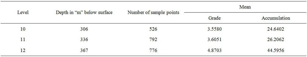
Table 1. Details of data.
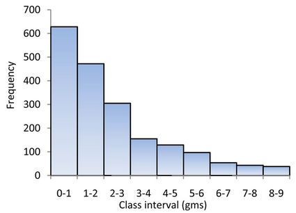
Figure 1. Histogram for grade (gm/tonne).
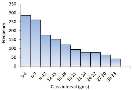
Figure 2. Histogram for accumulation (m-gms).
noise. Such time series could be broadly categorised a stationary or non-stationary. The stationary assumption implies that the probability distribution  is the same for all times—t, possessing a constant mean. In order to test for stationarity, the assay data were tested. A simple but robust method followed for testing of stationarity was as follows: Each level data was divided into three segments. The mean and variance were computed for each of the segments. Now a 10% of the first portion assay data were removed from the segment and to compensate this, a 10% assay data of first portion of the second segment was added to the first segment. For the second segment, 10% of the first portion of third segment was appended. The third segment is now short of 10% data and to compensate this, some extra data were added. The mean and variance were computed for this revised
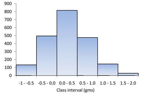
Figure 3. Histogram for the logarithms of grade (gm/tonne).
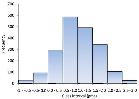
Figure 4. Histogram for the logarithms of accumulation (m-gms).
segment. It is observed that the mean and variances remained more or less the same conforming to the discrete process being weakly stationary. In order to analyse the stochastic characterization of the mineralization, three modeling frame works viz., Auto-regressive [AR (p)], Moving average [MA (q)] and Auto regressive and moving average [ARMA (p, q)]—were considered. The ARMA has both the AR and MA component. The “acf” and the “pacf” would give an indication as to the appropriate candidate models to be chosen. For the sake of completeness, brief details concerning the parameter estimation of these linear stochastic models and criteria adopted for choosing the appropriate model are given below.
3.1. Parameter Estimation
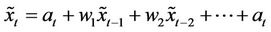
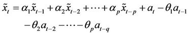
Following Box and Jenkins (1970, p. 9) linear random filter model is given by
 (1)
(1)
This can also be thought of as the representation of a stochastic process whose input is white noise distributed as  and output
  are parameters representing the weight coefficients. Since the process is found to be stationary,
  is the mean of the
  process. If the sampled estimate
  of the mean
  is subtracted from the time series, we have
 , and the process will therefore be considered as a zero mean process. Equation (1) implies that
  can be written alternately as a weighted sum of past values of the
 ’s plus an added shock. Thus
 (2)
(2)
The special cases of this model in which only the first p of the weights in non-zero may be termed as Auto regressive process of order “p”—[AR(p)]. It may be expressed as:
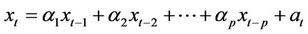 (3)
(3)
where  are used for finite set of weight coefficient; and where only the first “q” of the weights are non-zero, may be written as:
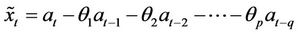 (4)
(4)
This is moving average process of order “q” that is MA (q). In practice, to obtain a parsimonious representation, it will be necessary to include both auto-regressive and moving average terms in the model. Thus, we have:
 (5)
(5)
Using the back-shift operator detailed by Box and Jenkins [7], this can be written as: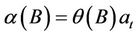 .
.
3.2. AR Process
The parameters of an AR model can be estimated by solving Yule-Walker equations [8,9]. The recursivescheme for estimate AR coefficients is detailed by Andersen [10].
3.3. MA (1) and ARMA (1, 1) Models
The MA (1) and ARMA (1, 1) models that follow (4) and (5) above are follows:
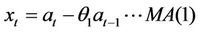 (6)
(6)
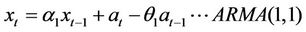 (7)
(7)
The estimations of parameters of the MA and ARMA processes is detailed by Box and Jenkins [7]. Tables 2 and 3 give the parameters of AR models with standard error for grade and accumulation respectively.
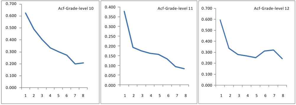
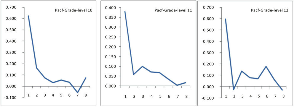
3.4. Auto-Correlation (acf) and Partial Auto-Correlation (pacf) Functions
In order to choose the appropriate candidate models by any of the approaches described above, the “acf” and the “pacf” of the process were examined as these are most essential in model identification. The auto-correlation coefficients  and “pacf” for different lags (k < N/4), where N is the sample size, were computed employing the standard formula [7], In all the cases, the “acf” followed a near damped exponential pattern while the “pacf” followed a cut-off pattern indicating that the process could be AR. The model to be selected could be
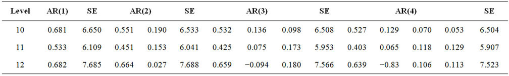
Table 2. Parameters of AR models with standard error for grade.
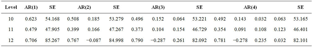
Table 3. Parameters of AR models with standard error for accumulation.
recognised by the application of statistical significant tests based on variance of acf:
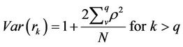 (8)
(8)
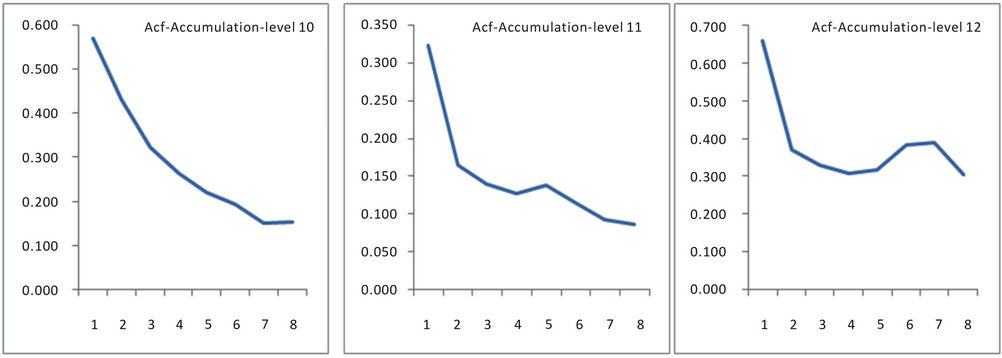
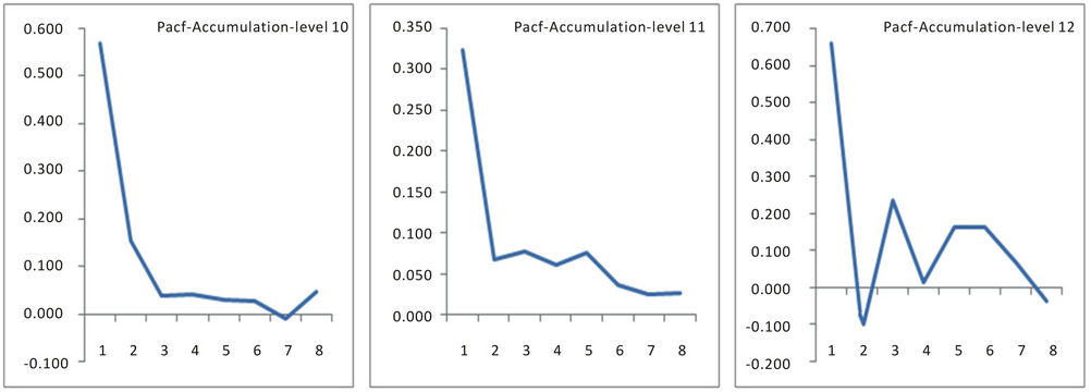
and the variance of pacf: 1/N [7]. Figures 5 and 6 show the acf and pacf for levels 10, 11 and 12 in respect of grade while Figures 7 and 8 show the acf and pacf for levels 10, 11 and 12 in respect of accumulation.
4. Structural Analysis
The variables under consideration were weakly stationary; that is their mean and variances are constant. A stationary random function is homogeneous and self repeating in space. Strict sense stationarity requires all the moments to be invariant under translation but this cannot be verified when the experimental data are limited. Usually the first two moments, mean and covariance are expected to remain constant. This is called weak or second order stationarity. However these assumptions related to weak stationarity may not always be satisfied. In the case, where there is a marked trend, the mean value cannot be assumed to be constant. Further, in some cases the covariance need not exist. Hence, this hypothesis needs to be further weakened [11]. Under the intrinsic hypothesis, we assume that the increments of the function  are stationary.
That is, for any vector h. The increment 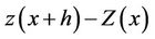 has a mean and a variance which are independent of x. That is
 ![]() or
or ![]() and
and ![]() , a finite value which is independent of X. This function
, a finite value which is independent of X. This function  is called semivariogram. It is the fundamental tool for spatial structural interpretation of phenomenon as well as for estimation—
 (a) (b) (c)
Figure 5. Acf of grade for levels 10, 11 and 12.
 (a) (b) (c)
Figure 6. Pacf of grade for levels 10, 11 and 12.
 (a) (b) (c)
Figure 7. Acf of accumulation for levels 10, 11 and 12.
 (a) (b) (c)
Figure 8. Pacf of accumulation for levels 10, 11 and 12.
known as kriging. Notable authors in this line of approach are Matheron, Armstrong, Clark, Journel and Hujibregts, Royale [11-14]. Sarma applied this approach to gold mineralization in respect of Zone-I, and Oakley’s reefs of Hutti gold mines.
4.1. The Semi-Variogram
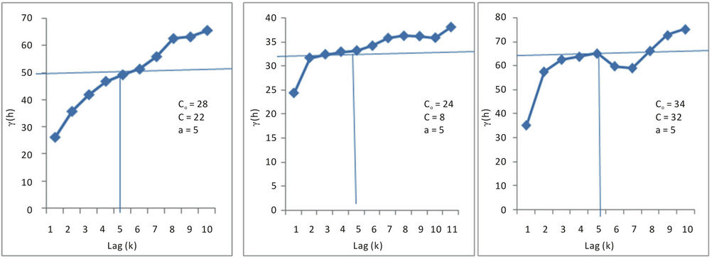
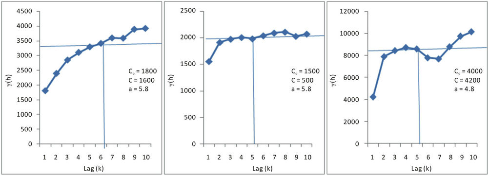
In order to study the spatial structure of mineralization, experimental semi-Variograms were constructed for each of the levels 10 - 12 of the Hutti gold mine. The experimental semi-Variogram was spherical in nature. Therefore, spherical models were fitted. The spherical model has the following general form.
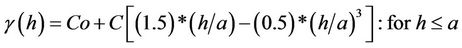
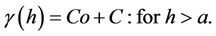
where :
: , and
, and  . Table 4 shows these spherical functions for the variables grade and accumulation. Figures 9 and 10 show these semi-variograms for grade and accumulation with N as sample size together with model parameters.
The details of values for the parameters C0 = nugget effect, a = range and sill Co + C are given in the Table 4.
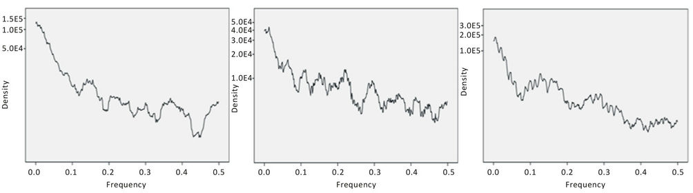
4.2. Spectrum Analysis (Frequency Domain)
According to Hayakin (1983), in the characterisation of a spectral density, spectrum analysis is often preferred to the auto-correlation function because of a spectral representation may reveal such useful information as hidden periodicities or closed spectral peaks. The great interest in the computation of spectrum shown by many scientists is largely motivated by possible presence of sharp peaks of considerable physical importance. Different methods such as Blackman-Tukey, Fast Fourier Transform (FFT), Maximum Entropy Method (MEM) and Maximum Likely
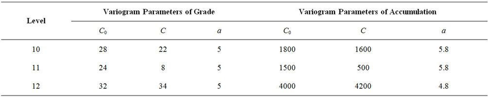
Table 4. Details of variogram parameters for levels 10, 11 and 12.
 (a) (b) (c)
Figure 9. Semi-variogram of grade for levels 10, 11 and 12.
 (a) (b) (c)
Figure 10. Semi-variogram of accumulation for levels 10, 11 and 12.
hood Method (MLM) exist for computation of spectral densities. The advantage with MEM is that the windowing problem which is present in the other methods can be overcome [15]. The basic idea is to choose the spectrum which corresponds to the most random time series whose “acf” agrees with a set of known values. MEM estimates the spectra reasonably well, particularly when the length of the available time series is limited. For a linear process the spectral density estimate is given [16] by
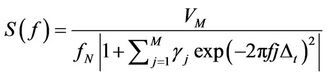 (9)
(9)
where  is a constant representing the updated variance of the series, and
  are prediction coefficients that are determined from the data;
  is the frequency and
  is the Nyquist frequency:
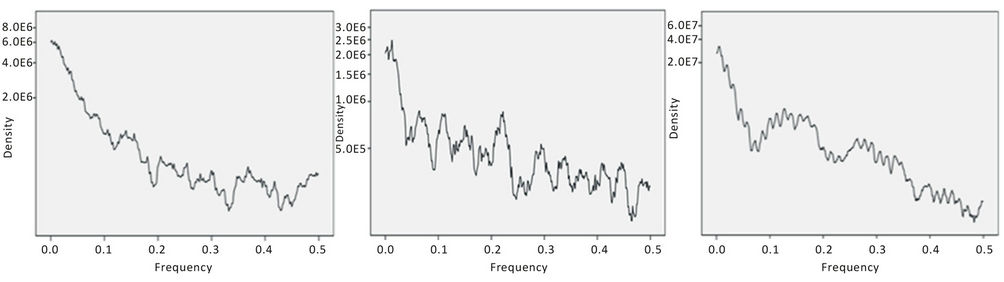
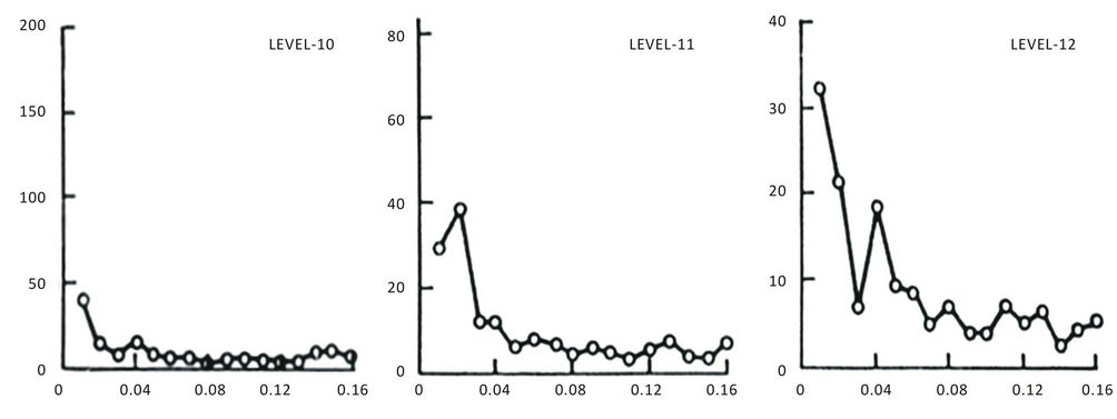
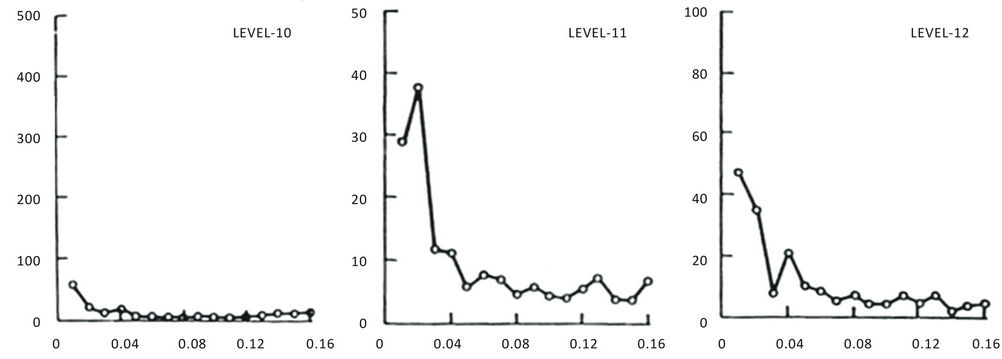
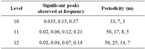
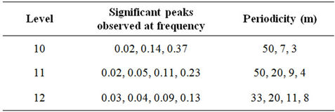
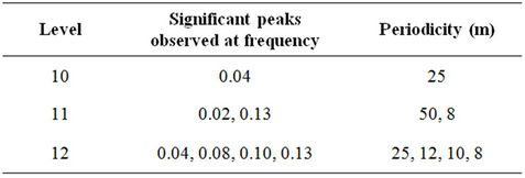
 . A common method of obtaining estimates of is by solving YuleWalker (Y-W) equations [8,9] which involve computation of auto-covariances. Figures 11 and 12 show the spectra for levels 10, 11 and 12 for grade and accumulation by FFT while Figures 13 and 14 show the spectra for levels 10, 11 and 12 for grade and accumulation by MEM method.
Based on the spectra the observed periodicities are as follows:
 (a) (b) (c)
Figure 11. Spectra for grade by FFT for levels 10, 11 and 12.
 (a) (b) (c)
Figure 12. Spectra for accumulation by FFT for levels 10, 11 and 12.
 (a) (b) (c)
Figure 13. Spectra for grade by MEM for levels 10, 11 and 12.
 (a) (b) (c)
Figure 14. Spectra for accumulation by MEM for levels 10, 11 and 12.
Grade-periodicity: FFT
Accumulation-periodicity: FFT
Grade-periodicity: MEM
Accumulation-periodicity: MEM
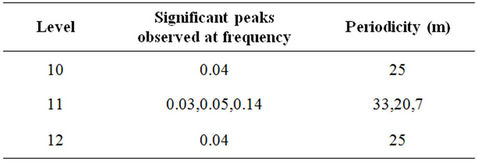
Table below shows common periodicities observed by FFT and MEM methods in respect of grade and accumulation.
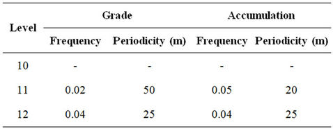
5. Conclusion
The distribution of grade and accumulation in respect of gold mineralization in the Strike Reef (Footwall branch) of Hutti gold mines follow approximately a lognormal distribution. This inference is significant as the mines are shallow in depth, usually not exceeding 600 m. Based on acf and pacf, the process is identified as AR. The AR parameters were worked for the grade and accumulation in respect of levels 10, 11 and 12. Based on standard error, a fourth order AR is was found to be appropriate. Structural analysis revealed that the semi-variograms are spherical in nature, both in respect of grade and accumulation. Spectrum analysis by FFT and MEM showed common periodicities for grade and accumulation for every 50 m for level 11 and for every 25 m for level 12. Similarly the periodicities are 25 m for level 11 and 12 both in respect of grade and accumulation.
6. Acknowledgements
The first author sincerely thanks to UGC-BSR for providing the Fellowship. The second author thanks to the Chairman and Managing Director of Hutti gold mines Limited for permission to collect the relevant assay data for research purposes.
REFERENCES
- D. D. Sarma, “A Statistical Appraisal of Ore Valuation. (With Application to Kolar Gold Fields),” Series No. 157, Andhra University Press, Waltair, 1979.
- D. D. Sarma, “Stochastic Modeling of Gold Mineralisation in the Champion Lode System of Kolar Gold Fields (India),” Mathematical Geology, Vol. 22, No. 3, 1990, pp. 261-279. doi:10.1007/BF00889889
- D. D. Sarma, “Geostatistics with Applications in Earth Sciences,” 2nd Edition, Capital Publishing Company, New Delhi, 2009. doi:10.1007/978-1-4020-9380-7
- D. D. Sarma and G. S. Koch, “A Statistical Analysis of Exploration Geochemical Data for Uranium,” Mathematical Geology, Vol. 12, No. 2. 1980, pp. 99-114. doi:10.1007/BF01035242
- B. K. Sahu, “Time Series Modeling in Earth Sciences,” Oxford & IBH Publications, New Delhi, 2003, p. 24.
- B. K. Sahu, “Statistical Models in Earth Sciences,” BS Publications, Hyderabad, 2005, p. 210.
- G. E. P. Box and G. M. Jenkins, “Time Series Analysis: Forecasting and Control,” 2nd Edition, Holden-Day, San Francisco, 1970, p. 5.
- G. U. Yule, “On a Method of Investigating Periodicities in Disturbed Series in Spectral Reference to Wolfer’s Son Spot Numbers,” Philosophical Transactions of the Royal Society, Series-A, Vol. 226, 1927, pp. 267-298. doi:10.1098/rsta.1927.0007
- G. Walker, “On Periodicity in Series of Related Terms,” Philosophical Transactions of the Royal Society, Series-A, Vol. 131, 1931, pp. 518-532.
- N. Andersen, “On the Calculation of Filter Coefficients for Maximum Entropy Spectral Analysis,” Geophysics, Vol. 39, No.1, 1974, p. 6.
- M. Armstrong, “Common Problems Seen in Variograms,” Mathematical Geology, Vol. 16, No. 3, 1984, pp. 305- 313. doi:10.1007/BF01032694
- G. Matheron, “Principles of Geo-Statistics,” Economic Geology, Vol. 58, 1963, pp. 1245-1266. doi:10.2113/gsecongeo.58.8.1246
- I. Clark, “Practical Geo-Statistics,” Applied Science Publishers Ltd., London, 1979, p. 129.
- A. G. Royle, “How to Use Geo-Statistics for Ore Reserve Classification,” World Mining, Vol. 30, 1977, pp. 52-56.
- S. Hayakin, “Introduction in Non-Linear Methods of Spectral Analysis,” Topic in Applied Physics, Vol. 34, 1983, p. 263.
- T. J. Ulrych and T. N. Bishop, “Maximum Entropy Spectral Analysis and Auto-Regressive Decomposition,” Reviews of Geophysics and Space Physics, Vol. 130, No. 1, 1975, pp. 183-200. doi:10.1029/RG013i001p00183