Advances in Remote Sensing
Vol. 2 No. 2 (2013) , Article ID: 33222 , 19 pages DOI:10.4236/ars.2013.22020
Monitoring Wheat and Rapeseed by Using Synchronous Optical and Radar Satellite Data—From Temporal Signatures to Crop Parameters Estimation
Centre d’Etudes Spatiales de la Biosphère (CESBIO), Université de Toulouse, Toulouse, France
Email: remy.fieuzal@cesbio.cnes.fr
Copyright © 2013 Rémy Fieuzal et al. This is an open access article distributed under the Creative Commons Attribution License, which permits unrestricted use, distribution, and reproduction in any medium, provided the original work is properly cited.
Received April 10, 2013; revised May 9, 2013; accepted May 17, 2013
Keywords: TerraSAR-X; Radarsat-2; Alos; X-Band; C-Band; L-Band; SAR; Formosat-2; Spot-4/5; Optical; Wheat; Rapeseed; Crop Height; Leaf Area Index
ABSTRACT
This paper investigates the sensitivity of multi-temporal SAR data acquired at different frequencies (X-, Cand L-bands), polarizations (HH, VV, VH and HV) and incidence angles (from 24˚ to 53˚) during the growing season of two winter crops (rapeseed and wheat). This study was part of a multi-sensor crop-monitoring experiment that was performed from February to November 2010 (MCM’10). During the experiment, dense series of satellite data were acquired in microwave, optical and thermal domains (more than 150 images were provided by TerraSAR-X, Radarsat-2 Alos, Formosat-2, Spot-4/5 and Landsat-5/7) were synchronous with ground measurements over an agricultural area located in southwestern France, near Toulouse. An angular normalization of radar signals is first performed for each crop type at Xand C-bands by using a dense temporal satellite series and the complementarity provided by microwave and optical data. The results show that the angular sensitivity of radar backscatter decreases with the increase of the vegetation index (from 0.4 dB.˚−1 over bare soils to 0.05 dB.˚−1 for fully vegetated fields). Lower angular sensitivity is observed at X-band (compared to C-band), and for the cross-polarized signal. Analyses of the temporal signatures of the radar backscatter show a well-marked signal dynamic at X-, Cand L-bands, depending on the crops and theirs associated phenological stages. During the stems elongation of wheat while the NDVI increases of 0.2, a dynamic of 10 dB is observed at X-band and at C-band with VV polarization. Interesting behaviors are also observed during the crop senescence with an increase of several dB (depending on the sensor configuration), while the NDVI decreases of 0.5. Over rapeseed, cross-polarized backscatters offer promising dynamic of 6 dB during the seed development, while the NDVI saturates at maximum values. The use of radar signals, in complement of optical, for crop parameters monitoring is achieved in terms of leaf area index and crop height estimations. Over rapeseed, best correlations between crop parameters and radar signals are obtained at C-band, by combining coand cross-polarized backscatters (R2 > 0.61). Over wheat, best results are achieved by using X-band data (R2 > 0.64).
1. Introduction
In a global context of climate change, as evidenced by increased temperatures [1], modifications of precipitation patterns [2], and population growth (with a rate of 1.1% per year in 2011), those who work in agriculture have an imperative to implement production techniques that will achieve sufficient yields while minimizing the waste of natural resources (water, food, etc.). Effective management of the means of production requires understanding of the processes that govern agricultural ecosystems while identifying adequate adaptive responses to change [3-5]. Crops represent a key component of these ecosystems at the interface between the soil and the atmosphere. They are associated with significant temporal dynamics, and strong spatial heterogeneity that is reinforced by differences among cultivated species, resulting in profound changes during the growing season. Furthermore, crops have direct or indirect effects on different surface balances (carbon, nitrogen, water or energy) that are closely linked to cultural practices (tillage, fertilizer, irrigation and residue management) [6-9]. Those past analyses have been mainly conducted at local scale, over a limited number of fields, and need to be extrapolated over a larger agricultural area to estimate the overall impacts of crop management practices. Because of their high coverage capacity (several square kilometers) and temporal revisits, remote sensing satellites can be used as a suitable tool for monitoring land surface changes [10-12]. Within the range of onboard sensors in different satellites, those that function in the microwave domain have the twofold advantage of not being disturbed by atmospheric conditions [13] (except for large convective systems) while offering a high degree of sensitivity to surface parameters [14].
In the microwave domain, many studies have been conducted with ground-based antennas, airborne flights and spacecraft missions (ERS-1/2, EnviSat, Radarsat-2 and others) associated with ground-measurement campaigns. These studies have addressed the sensitivity of multi-frequency, multi-incidence and multi-polarization data to surface parameters. With regard to agricultural areas, measurements have been performed on contrasting surfaces (bare soil and vegetated fields), allowing the distinction between the parameters related to soil and those related to crops. Following the soil contribution, influences from different levels of topsoil moisture, surface roughness and texture on backscattering coefficients have been widely analyzed since the 1980s [15-20] showing the importance of the sensor configurations (wavelength, incidence angle or polarization states). Studies addressing the sensitivities of vegetation parameters are mainly based on data acquired during specific phenological stages, at local scale [16,21,22]. It is thus difficult to generalize radar signal behavior over the entire crop cycle, especially at landscape scale where surface conditions can be strongly contrasted (soil and vegetation managements, soil type ...). Few studies include both analysis during the entire cycle of culture and a large number of agricultural parcels by using satellite data.
According to the wheat and rapeseed monitoring, results are mainly based on data acquired at C-band. At this frequency, the temporal behaviors of wheat presented in different studies [23,24] show similar global trends, although the radar signal behaviors are specifics to the study site. Furthermore, interest of using copolarized backscatter ratio  has been pointed over wheat for biomass monitoring. At X-band, no temporal analyses have been achieved over wheat or rape by using satellite data. Nevertheless, [25] showed promising results for monitoring wheat by using ground-based Xband antenna. Until now, the comparison of the radar signal sensitivities observed at the different microwave frequencies still appears challenging, as measurements are performed over different studied sites where surface and climatic conditions are often contrasted.
Studies based on the use of satellite data are dependent on ongoing missions. Recent studies have developed multi-sensor approaches for agricultural management purposes (irrigation surveys, agricultural soil management or natural grassland monitoring) by underscoring the importance of combining optical and radar images [26-31]. In microwave domain, the launch of TerraSAR-X and Alos satellites has enabled the use of multifrequency radar signals to monitor crops such as sugarcane, corn and soybean, or agricultural surface parameters [32-35]. Those missions at Xand L-bands, supplement C-band data available from the nineties with the launch of ERS-1. However, it is still challenging to acquire synchronous multi-sensor time series, in order to analyze satellite data sensitivity over comparable surface conditions.
In this context, the objective of the present study is twofold: 1) to analyze the temporal behaviors of radar and optical satellite signals quasi-synchronously acquired over two winter crops (rapeseed and wheat) from the growing period until harvest, and 2) to compare the sensitivity of those data to crop parameters (leaf area index and height). To this end, this paper is structured as follows: Section 2 presents an overview of the study site. The ground measurements and satellite signal processing steps are described in Section 3. The methodology is presented in Section 4. Section 5 presents the results of the SAR angular normalization and the time series analyses of satellite data (optical and radar) acquired over wheat and rapeseed. This section also includes the empirical relationships that were estimated for radar backscatter and crop parameters (crop height and leaf area index).
2. Study Site
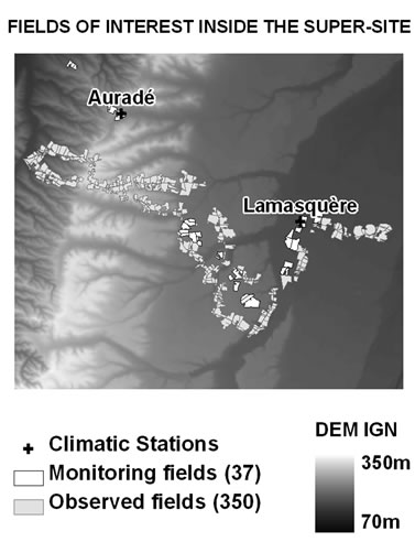
This study was carried out over a 15 by 15 km2 area, which was defined as a supersite and located in southwestern France in the Midi-Pyrénées region near Toulouse (coordinates for the center of the area are 43˚29'36"N, 01˚14'14”E) (Figure 1). The supersite includes 387 fields and two meteorological stations (near the villages of Auradé and Lamasquère). This dense network of observations and measurements is considered to be representative of the whole supersite in terms of soil and vegetation characteristics.
The eastern part of the supersite is quite flat, with slopes lower than 1˚, in contrast to the western part, where the slope is at a mean of 4.5˚. Soil types are mainly silty loam, with the clay, silt and sand contents respectively ranging from 9% to 58%, from 22% to 77% and from 4% to 53% [36].
The site’s meteorological conditions are dictated by a temperate climate (Figure 2). For the year 2010, records show that approximately 20% of the annual rainfall, which is close to 600 mm, occurs in the month of May.
 (a)
(a)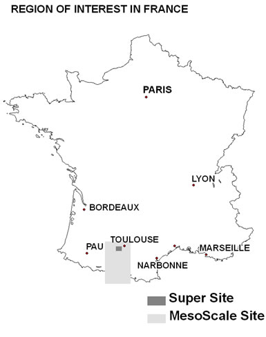 (b)
(b)
Figure 1. Location of the study sites in southwestern France showing the 3 embedded spatial scales (mesoscale, supersite and the two local sites of Lamasquère and Auradé). The locations of the 387 studied fields are presented in Figure 1(b) over the supersite, which were superimposed on the digital elevation model provided by the French national geographic institute (IGN).
Figure 2. Ombrothermic diagram of the year 2010. Monthly mean air temperatures (in gray) and cumulative precipitations (in black) are taken from the meteorological station at Lamasquère.
There is an amplitude of almost 20˚C between the extreme mean air temperatures observed in January (3.5˚C) and July (22˚C).
The supersite is mainly covered by crops (56.8%), grasslands (32.1%), sparse forests (7.9%), urban areas (2.4%) and water bodies (0.8%). In this paper, there is a focus on the two principal winter crops of the study area —rapeseed and wheat—for which the field size and the local slope are respectively ranged from 0.3 to 24 hectares and from 0˚ to 5.3˚. For rapeseed, the sowing period occurs from September to October of 2009, and the harvest occurs from June to July of 2010. For wheat, various varieties are sown from October to December 2009 and harvested from June to July of 2010.
3. Ground and Satellite Data
The data presented below are part of the Multi-sensor Crop Monitoring experiment that was conducted throughout the year 2010 [36].
3.1. Ground Data
Ground measurements consist of qualitative (observations) and quantitative (in-situ meas-urements) parameters, and the collection is performed over 350 and 37 fields, respectively (Figure 1). The data are collected at each satellite overpass with a mean lag of 1 day.
Land use observations are collected over the 350 “observing fields”. They consist of determining the crop types (wheat, rapeseed, corn, etc.) and agricultural practices (irrigation, sowing, tillage, harvesting, etc.). The dates of sowing and harvesting are used in this study for twelve fields of rapeseed and seventy fields of wheat.
Regular qualitative and quantitative measurements are collected over the 37 “monitoring fields”. Four fields of rapeseed and thirteen fields of wheat are monitored (Table 1). Vegetation measurements consist of the determination of the crop phenological stages and heights. Soil measurements include the top soil moisture collection (using mobile Theta-probes sensors), and surface roughness (using a 2 meter profilmeter).
Figure 3 shows the temporal behaviors of the crop heights together with examples of the main specific crop phenological stages that were described by [37]. In the rapeseed fields, values of height range from 20 to 200 cm. Maximal values are observed during flowering, after which the height decreases as a result of progressive bending of the vegetation. Crop height heterogeneities are observed from flowering until harvest, with differences between minimal and maximal values ranging from 10 to 40 cm. The wheat fields have mean crop heights ranging from 10 to 90 cm, with maximal values during grain heading. Mean values are associated to variations, ranging from 13 to 45 cm, caused by both the discrepancy in the crop growth and the different wheat development.
According to soil moisture, regular top soil moisture (TSM) measurements are collected using mobile sensors. A calibration function is first established between the signals delivered by the sensors (in milliVolt, mV) and the volumetric measurements performed over six soilcontrasted sites [36].
 (1)
(1)
This relationship is used to transform in percent (or m3 by m−3) the sensor’s signal collected along transects at each satellite overpass. In this study, the mean fields’ values are derived from at least 15 measurements. Dry and wet top soil moisture conditions are observed, with values ranging from 5% to 34% on the rapeseed fields, and from 5% to 37% on the wheat fields (Table 1).
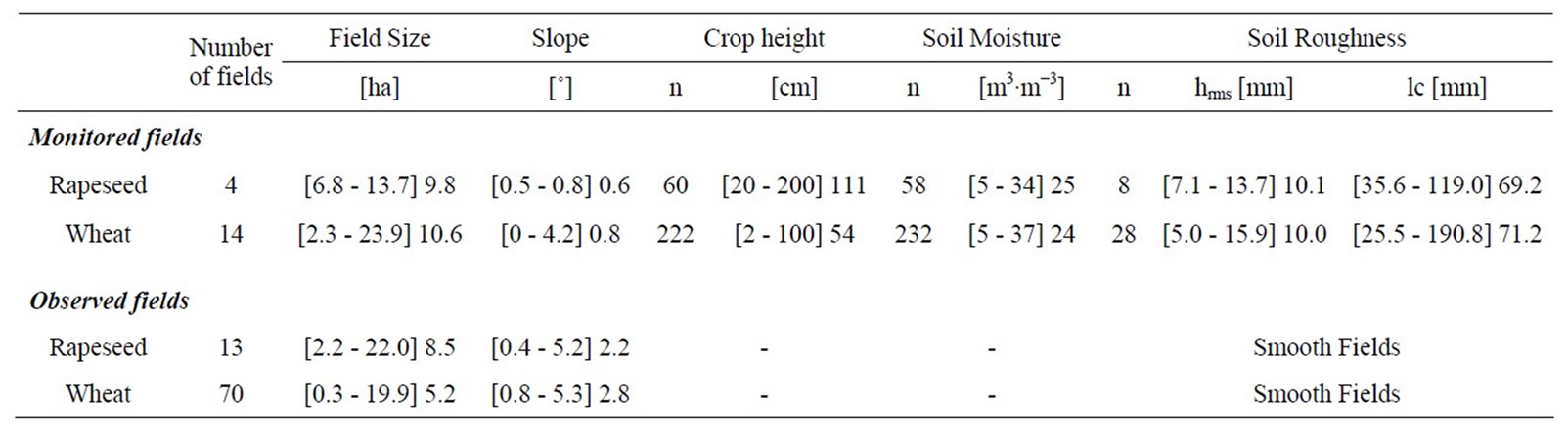
Table 1. Description the measurements performed over the observed and the monitored fields. According to the quantitative parameters, the numbers of measurements (n) are given together with the range (into brackets) and the mean values.
 (a)
(a)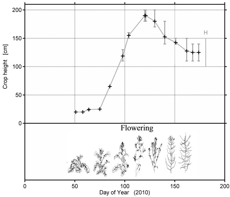 (b)
(b)
Figure 3. Crop height values (minimum, maximum and mean) collected over rapeseed (a) and wheat (b) fields together with specific crop phenological stages. Vertical gray lines and the letter “H” indicate the harvest day.
Surface roughness is collected after the crop sowing (along and perpendicular to the row direction). The height rms (hrms) and the correlation length (lc) are derived from each 2 meters roughness profile. Wheat and rapeseed fields are characterized by a mean hrms of 10 mm and a mean lc of 70 mm. During the crop growth cycle, these smooth surface roughness conditions are considered stable as no tillage events are performed. At landscape scale, these levels of roughness are identified as “smooth fields” (Table 1).
Climatic data (including air temperature, solar radiation, relative humidity, wind speed, rainfall, etc.) are collected semi-hourly by two meteorological stations (Figure 1). Rainfall time courses are displayed below, with the use of the nearest station regardless of the field under study.
3.2. Satellite Data
Satellite acquisitions are regularly planned and acquired during the year 2010. They are taken at a high spatial resolution (less than 20 m) from January to July (Figure 4). Microwave data are acquired quasi-synchronously by TerraSAR-X (TS-X), Radarsat-2 (RS-C) and Alos (AP-L) at three different wavelengths (3.1, 5.5 and 23.6 cm, respectively). Twenty-one images are provided by TerraSAR-X, 15 by Radarsat-2 and 7 by Alos. In the optical domain, Formosat-2 (FS-2) and Spot-4/5 respectively provide 7, 6 and 6 images, during the same period.
3.2.1. Optical Data
Formosat-2 is a Taiwanese satellite that was launched in May 2004 [38]. This satellite carries an optical sensor that provides images in four narrow wavelengths, ranging from 0.45 to 0.90 µm, that correspond to blue, green, red and near-infrared ranges. All the images are acquired with the same viewing angle (±45˚) by using the multispectral mode, which is characterized by a spatial resolution of 8 m.
Spot-4 and Spot-5 are European satellites that were

Figure 4. Satellite acquisition dates as performed by TerraSAR-X (with Spotlight ▼ and Stripmap ▲ modes), Radarsat-2 (●) and Alos (with fine-beam single polarization ■ and fine-beam dual polarization ♦ modes) in the microwave domain. Optical images are provided by Spot-4/5 (×) and Formosat-2 (+). According to the SAR acquisitions, the incidence angle (numbers on the top or bottom of the different markers) and the orbit (ascending in black, descending in white) are indicated for each image.
launched in March 1998 and in May 2002, respectively [39]. These satellites have optical instruments that operate in four different spectral bands ranging from 0.50 to 1.75 µm and corresponding to green, red and nearand medium-infrared wavelengths. The images are acquired with two different incidence angles (75˚ and 102˚) using the multispectral mode. The images provided by Spot-4 and Spot-5 are characterized by spatial resolutions of 20 and 10 m, respectively.
All optical data are processed with a multi-temporal algorithm to 1) detect clouds and their shadows on the soil and 2) correct for atmospheric disturbances (i.e., aerosol effects) by applying the method developed by [40], which is based on the assumption that surface reflectances and aerosol optical properties vary differently according to time and location. Those data are then used to derive two vegetation indexes: the NDVI and MTVI2. The Normalized Difference Vegetation Index (NDVI) is computed by using spectral bands in red and near-infrared [41]. The NDVI is used in the backscatter angular correction step and compared to radar backscatters behaviors (which are presented below and in Section 4). The Modified Triangular Vegetation Index (MTVI2, [42]) is derived from green, red and near-infrared spectral bands. The MTVI2 is used to derive the leaf area index (LAI) using an empirical relationship as proposed by [43].
3.2.2. Radar Data
TerraSAR-X is a German earth observation satellite that was launched in June 2007 [44]. The Synthetic Aperture Radar (SAR) instrument onboard the satellite operates at X-band (f = 9.65 GHz, λ = 3.1 cm). All images are acquired with the same polarization state (HH) at incidence angles ranging from 27.3˚ to 53.3˚ in order to increase the repetitiveness of observations offered by the initial 11-day orbital cycle. Two acquisition modes are combined: the StripMap (SM) and SpotLight (SL), which are characterized by pixel spacing of approximately 3 and 1.5 m, respectively.
The Canadian satellite Radarsat-2 was launched in December 2007 [45]. It has a SAR instrument operating at C-band (f = 5.405 GHz, λ = 5.5 cm). The orbital cycle is 24 days, but the combination of different orbit and incidence angles allows for an increase in the number of possible acquisitions per cycle. The images are all acquired with the full quad-polarization mode (Fine QuadPol), which delivers images at HH, VV, HV and VH polarizations. The incidence angles range from 24˚ to 41˚, with a pixel spacing equal to 5 m.
Japan’s Advanced Land Observing Satellite (Alos) was launched in January 2006 [46]. Alos carries two optical instruments and a Phased Array L-band Synthetic Aperture Radar (PALSAR) instrument operating at L-band (f = 1.27 GHz, λ = 23.6 cm). PALSAR operates in five different pre-selected and mutually exclusive observation modes with a 46-day orbital cycle. For the present study, the images are acquired at the same incidence angle (~38.7˚) with fine-beam single polarization (FBS at HH polarization) and fine-beam dual polarization (FBD, at HH and HV polarizations). The pixel spacing of FBS and FBD products are respectively equal to 6.25 and 12.5 m.
Backscattering coefficients are derived from the different microwave products via the following two main steps: a radiometric calibration is first applied, and all images are then geo-referenced using ortho-photos provided by the French national geographic institute (IGN).
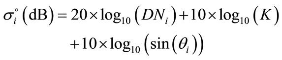
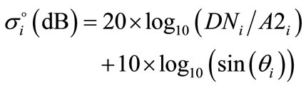
The radiometric calibration of TerraSAR-X images is based on a procedure described by [47] using Equation (2). Radarsat-2 and Alos images are calibrated using NEST software [48] by following Equations (3) and (4) [49].
 (2)
(2)
 (3)
(3)
 (4)
(4)
Backscattering coefficients (˚) are derived from the digital number (DN) of the pixel i, the calibration factor (K) and the incidence angle (θ) for TerraSAR-X and Alos. For Radarsat-2, the gain (A2) comes from the product data table.
Satellite data are geo-referenced by using aerial IGN ortho-photos (with a resolution of 50 cm). Ortho-photos are first resized according to the resolution of the image, and then 70 reference points are taken between the base (IGN ortho-photos) and warp (satellite data) images. The geo-location accuracy is on average lower than 2 pixels considering the different products.
4. Methodology
Figure 5 describes the method used to obtain comparable radar and optical signals for monitoring agricultural surfaces. Satellite data are averaged over the different fields with respect to their shapes and analyzed considering the temporal behaviors and the sensitivity to crop parameters.
The first step consists in calibrating radar images and in correcting optical image from the atmospheric perturbation. All images are then geo-referenced and satellite signal extracted. According to SAR signals, an angular normalization is then applied to the backscattering coefficients to analyze the normalized temporal signatures of wheat and rapeseed, at Xand C-bands. No angular correction is applied at L-band because all images are acquired with the same incidence angle (~38.7˚).
The temporal behaviors of optical and radar signals are finally analyzed and confronted to synchronous surface measurements. The sensitivities observed at the different frequencies (X-, Cand L-bands) and polarizations (HH, VV, HV and VH at C-band) are described over one “monitored field”. These multi-temporal trends, observed over rapeseed and wheat, are analyzed at landscape scale with the signals collected over the “observed fields”. Lastly, the sensitivity of the satellite data to crop parameters (crop height and leaf are index) is established, defining linear relationship until the signal saturation.
5. Results and Discussion
5.1. Angular Normalization of SAR Backscatters
Previous studies have shown the strong influence of incidence angle on backscattering coefficients during particular crop stages for contrasted soil conditions [16, 22,24,50].
In this context, it becomes necessary to develop a method to take into account the angular sensitivity of the radar signal during the entire cultural season. The proposed approach is based on the empirical relationship between the NDVI value and the backscattering coefficient differences that are estimated from two successive angular-contrasted images (as expressed in dB by degree, dB.˚−1) (Equation (5)). Relationships are established for each crop type by separating frequencies and polarization states. Those relationships are then used to obtain normalized backscattering coefficients with the same incidence angle (~38.7˚, such as Alos images).
 (5)
(5)
 represents the difference in backscattering coefficients between two successive radar images; NDVI is
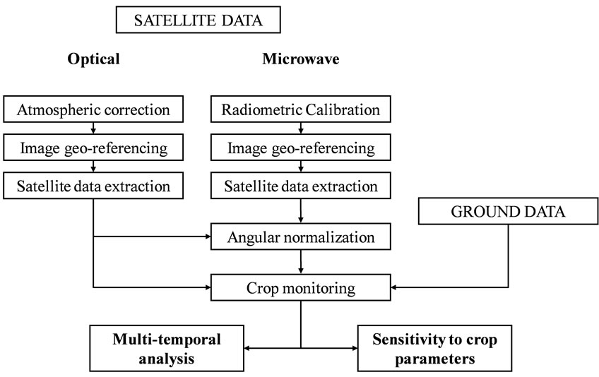
Figure 5. Synopsis of images and ground data processing involved in multi-temporal and crop sensitivity analysis.
derived from optical images. Letters a, b and c represent empirical parameters.
This proposed method satisfies the assumptions that within the microwave domain, the selected images must be the closest in time (to minimize disturbances from surface changes) and with the largest gap relative to the incidence angle (to maximize the effect of the incidence angle). For TerraSAR-X, the pairs of images acquired with a difference of ~26˚ (between acquisitions performed at 27.3˚ and 53.3˚) and with a one-day lag are retained. For Radarsat-2, the difference between the incidence angles for two successive images is smaller (~14˚ at a minimum, between acquisitions at 26˚ and 40˚), and the maximal time interval is 13 days. In this case, a special attention is paid to the top soil moisture difference between the pairs of images which is lower than 4% or m3 by m−3 (for TerraSAR-X images, this difference is lower than 2% or m3 by m−3).
The NDVI is derived from the nineteen optical images acquired between January and July. To match them with microwave acquisitions, the NDVI values are daily-interpolated with the assumption that changes in crop growth are gradual during short periods (the mean interval between two optical acquisitions is close to 9 days). Depending on the satellite sensor, the NDVI values are compared for quasi-synchronous acquisitions between Spot-4 and -5 and Formosat-2 (acquired on the 9th and 10th of April). The results show a strong correlation between NDVISPOT-4, NDVISPOT-5 and NDVIFORMOSAT-2, with a coefficient of determination that is superior to 0.99 and a relative RMSE that is inferior to 8%. Consequently, all subsequent NDVI values are merged, regardless of the satellite sensor.
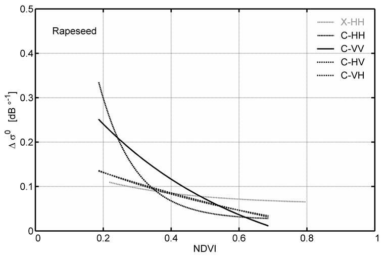
Figure 6 shows the relationships that are obtained between the angular sensitivity of the radar backscatter and the NDVI values for rapeseed and wheat. The results reveal different behaviors linked to both radar image characteristics (frequency and polarization) and crop type. Higher sensitivity is observed at C-band (compared to X-band), especially at the HH and VV polarization states, with an exponential decrease as the NDVI increases. A lower sensitivity is observed at HV or VH polarization whatever the value of NDVI.
For low NDVI values (~0.2), the Δs˚ ranges from 0.15 to 0.38 dB.˚−1 depending on the backscatter polarization sensitivity to bare soil parameters (topsoil moisture and roughness). For NDVIs higher than 0.4, Δs˚ saturates below 0.1 dB.˚−1 whatever the crop type, the radar frequency and the polarization. The variation of angular response along with crop growth confirms and generalizes the observations that were made in previous studies [22,50].
Empirical parameter values (a, b and c) are displayed in Table 2 together with statistical indexes. Although the
 (a)
(a)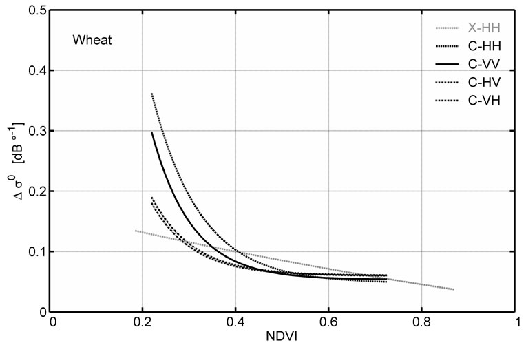 (b)
(b)
Figure 6. Empirical relationships between the Normalized Difference Vegetation Index (NDVI) and the difference in backscattering coefficients between two successive images that are acquired at high and low incidence angles (Δσ˚). Signal sensitivities are analyzed for rapeseed (a) and wheat (b) at X-band at HH polarization (in gray) and at C-band for full polarization (in black).
relationships are established by considering fields with contrasting cultural conditions (e.g., different crop varieties with contrasting row spacing, different row directions, etc.), their performances are acceptable and can be applied at landscape scale, with coefficients of determination (R2) ranging from 0.51 to 0.98 and a mean relative error (rRMSE) close to 30%. Cross-polarized backscatter is less sensitive to the incidence angle, which explains the lower accuracy observed (R2 ranged from 0.51 to 0.56).
The impact of the angular normalization on the backscattering coefficients acquired during the crop growth is illustrated on the Figure 7 by comparing the X-band signal before and after normalization. The difference is strongly marked due to the wide range of the acquisition’s incidence angles at this frequency (from 27˚ to 53˚). Before the angular normalization, the maximal difference observed between one day lag acquisitions is respectively equal to 3.37 and 2.25 dB, over wheat and
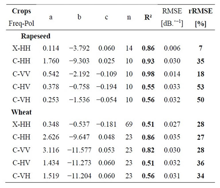
Table 2. Parameter values (a, b and c) used in empirical relationships for the angular correction performed at Xand C-bands (and corresponding polarizations states) together with the absolute and relative root mean square errors and the coefficients of determination (RMSE, rRMSE and R2, respectively).
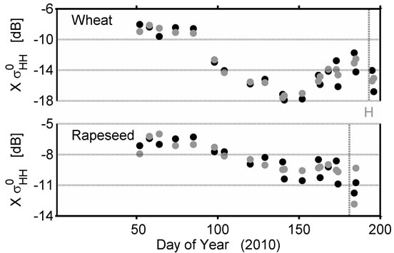
Figure 7. Temporal evolution of the backscattering coefficients acquired at X-band, over two fields cultivated with wheat and rapeseed, before the angular normalization (in black) and after (in grey).
rapeseed. After the angular normalization, this difference is respectively reduced to 0.70 and 0.16 dB. Furthermore, the maximal effects of the angular normalization are observed for the acquisitions performed at low (27˚) and high (53˚) incidence angles, for first and last phenological stages for which NDVI values are low.
5.2. Multi-Frequency Temporal Behaviors
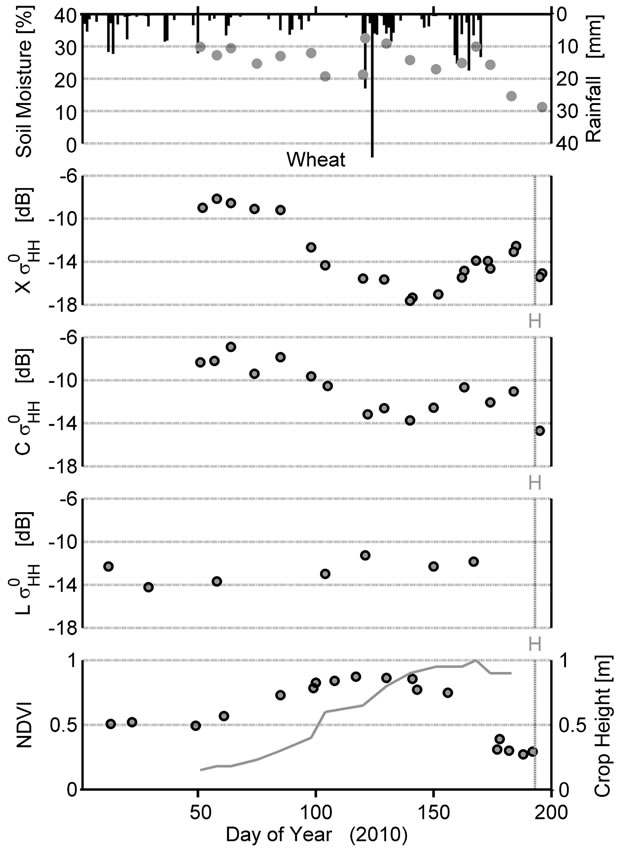
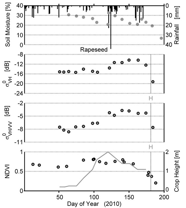
The temporal behaviors of multi-frequency (X-, Cand L-bands) backscattering coefficients at HH polarization are presented in the Figures 8 and 9 for rapeseed and wheat, respectively. Radar signals are plotted together with NDVI, crop height (m), top soil moisture (% volumetric) and rainfall events (mm). Figures 8(a) and 9(a) represent the temporal behaviors that are observed for one specific field of rapeseed and wheat, whereas Figures 8(b) and 9(b) highlight the general behaviors that are observed over several fields of the same crops. Whatever the field, the soil roughness is considered stable between sowing and harvest.
For the first satellite acquisitions performed at X and C-bands (20 February 2010, day 51 in the Figure 8(a)), the soil is covered by sparse vegetation characterized by a crop height of 20 cm and an NDVI close to 0.6. For the last dates (15 July 2010, day 196), the crops have been harvested and the surface is characterized by bare soil with stubbles. During the growing period, a higher signal dynamic is observed at X-band, with a difference between minimum and maximal values of approximately 4 dB. A lower difference between minimum and maximum values is observed at Cand L-bands, with 3 dB and 2 dB, respectively. Backscatter time courses show strongly contrasting behaviors for the different frequencies.
The X-band values for backscatter coefficients range between −6 and −10 dB. The maximum values are observed during the first phenological stages, and the minimum values are reached from the end of flowering to harvest. From days 74 to 140 (from flowering to pod appearance) the signal decreases linearly by approximately 3 dB. During this period, the NDVI presents values close to 0.75, with a little inflection which is caused by the crop flowering; the crop height reaches its maximum value and decreases to 1.5 m (this decrease is caused by the progressive inclination of the crop). According to the top soil moisture, values first decrease from 30% to 20%, and then increase after the first important rainfall event at day 121 (23 mm), without well marked effect on backscattering coefficients. From day 140 until harvest (corresponding to seed maturation), the backscattering coefficients stabilize around −10 dB. During this period, the radar signal is not affected by the decrease in crop height, the senescence of the crop or the top soil moisture variations. Figure 8(b) shows that the trend that is observed for one field is conserved over twelve fields throughout the crop cycle. Moreover, the low standard deviation observed at X-band (mean standard deviation close to 0.5 dB) indicates a strongly stable signal in time and space, regardless of the phenological stage or soil conditions (texture and moisture). At X-band, the signal is dominated by the vegetation component until its saturation. Only few contributions from soil are observed when vegetation is sparse (for first phenogical stages, until day 100).
Radar signal values at C-band range between −6 and −9 dB, with maximum values observed at days 150 and 163 and the minimum value at day 122, when the crop height reaches 2 m. A linear decrease is observed from days 85 to 122 (during the flowering stages and soil drying), followed by a period with higher backscatter values from day 129 until harvest (when the seeds grow). As observed, the increase of radar signal during this period
 (a)
(a)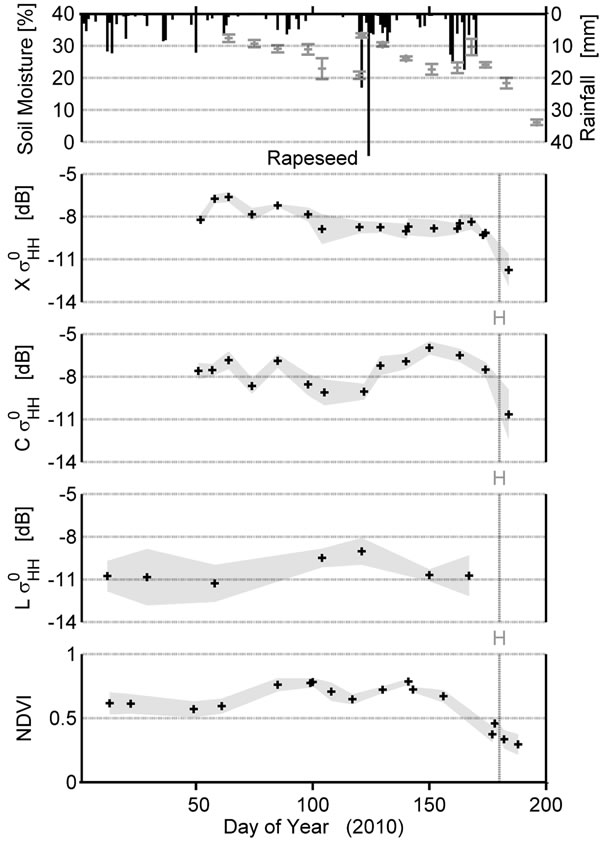 (b)
(b)
Figure 8. Temporal evolution of the backscattering coefficients acquired with X-, Cand L-bands at HH polarization over rapeseed fields. Over one monitored field, the backscatter is presented together with the NDVI derived from optical satellite data, crop height, soil moisture and rainfall events (a); At the landscape scale, the mean and standard deviation observed over twelve fields are used to delineate the satellite signal responses (b). Vertical gray lines and the letter ‘H’ indicate the harvest days.
 (a)
(a)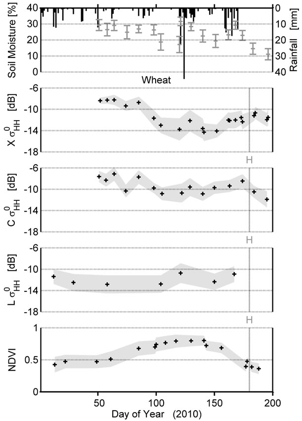 (b)
(b)
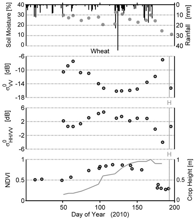
Figure 9. Temporal evolution of the backscattering coefficients acquired at X-, Cand L-bands at HH polarization over wheat. Over one monitored field, the backscatter is presented together with the NDVI derived from optical satellite data, crop height, soil moisture and rainfall events (a); At the landscape scale, the mean and standard deviation observed over seventy fields are used to delineate satellite signal responses (b). Vertical gray lines and the letter ‘H’ indicate the harvest days.
is not linked to the top soil moisture variations. The breakdown of scatter contributions is dominated by the ground, followed by vegetation with the development of different rapeseed organs (leaves, branches, petioles and pods) [22,51]. As for X-band, Figure 8(b) shows that the general trend observed for one field is conserved over twelve fields during the entire crop cycle. Nevertheless, the standard deviation is slightly higher than for X-band (the mean standard deviation values during the agricultural season is close to 0.5 dB at X-band and 0.7 dB at C-band), thus reinforcing the idea that the soil contribution is somewhat more significant at C-band over the vegetated area [16]. The slight increase in standard deviation values that is observed for acquisitions performed around day 100 (during crop flowering) may be explained by a discrepancy in crop phenological stages at the landscape scale.
At L-band, the backscattering coefficients show a linear increase during the growing period, followed by a slight decrease, occurring just after the crop inclination. The maximum value of −9 dB is reached at days 104 and 121, while contrasted soil moisture values are observed (23% against 33%) and vegetation height reaches its maximum. The minimum value of −11 dB is observed for the earliest crop stages (when the soil is covered by sparse vegetation, top soil moisture is high and soil roughness is low) and before harvest. Backscattering coefficients are in phase with the crop development, particularly with the crop height time course. The mean backscatter values are associated with standard deviations ranging from 0.4 to 2 dB over the twelve fields, which are higher than those observed at Xand C-bands. Maximum standard deviation values are observed for low biomass levels (for the first satellite acquisitions) and when the vegetation is drying (for the last acquisition). They are linked to the heterogeneous soil conditions (as a result of the moisture and roughness) mainly visible at L-band [15]. At the opposite, the dispersion of backscatters decreases over well-established crops.
On the monitored field of wheat (Figure 9(a)), soil is visible between crop rows for the first radar acquisitions at Xand C-bands (20 February 2010, day 51). At this time, the crop is characterized by a height of 15 cm and an NDVI close to 0.5. For the last dates, after harvest (15 July 2010, day 196), the soil is smooth and covered by straw residues and vertical stubble. The first two acquisitions are performed at L-band with lower vegetation heights (12 and 29 of January 2010).
Although the temporal behaviors are similar at Xand C-bands, the signal attenuation is more pronounced at X-band (10 dB against 6 dB of dynamic). Time courses are divided into three different periods during the crop growth cycle. From February to the end of March (days 51 to 85), the backscattering coefficients show only a few variations (in relation to topsoil moisture variations, especially at C-band), while the NDVI approaches the maximum values and crop heights slightly increases. Backscatter values linearly decrease from days 85 to 122 (during stem development), with a dynamic of approximately 9 and 6 dB at Xand C-bands, respectively. At the beginning of this period, the NDVI reaches its maximum value (~0.85) and saturates; the crop height increases from 0.3 to 0.9 m. Maximal top soil moisture values are observed during this period, inducing only little inflection of the backscattering coefficients after the highest rainfall event of the beginning of year 2010 (45 mm). Based on a radiative transfer model, [51] confirms that at C-band the breakdown of scatter contributions is first dominated by the ground before being masked by leaves and stems. Finally, from day 140 until harvest, the backscattering coefficients increase by approximately 5 and 3 dB at Xand C-bands, respectively. At the same time, the NDVI decreases during senescence (as the crop is drying). According to top soil moisture, values first approach the 30% after the rainfall period and decrease under 15% before harvest.
This temporal evolution is confirmed at the landscape scale over the seventy fields (Figure 9(b)), even when the satellite signals (in optical and microwave domains) show significant variability. Two interesting phenomena are observed at Xand C-bands. The first one involves a strong increase in the backscattering coefficient that occurs just after rainfall on day 120. In contrast to the rapeseed, this result shows that the backscattering signal is still influenced by a change in soil moisture under wheat (combined with the contribution of free water inside the wheat). The second interesting point concerns the significant standard deviation observed over wheat, regardless of the wavelength (mean standard deviation values during the agricultural season are close to 1.3 dB at Xand C-bands and 0.1 for NDVI). This variability is attributed to differences in crop development over the seventy fields. The main factor that explains the remote sensing signal variability are the biomass levels (as result of the combination of various cultivars, with different agricultural practices and heterogeneous soil properties) and a lag in crop sowing (more than one month between early and late sowing), which leads to a discrepancy in phenological stages.
At L-band, backscattering values range between −11 dB and −14 dB, with the maximum value observed after rainfall, associated to the maximal top soil moisture value (Figure 9(a)). The backscattering coefficients seem to be less linked to crop height than for rapeseed. Over the seventy fields (Figure 9(b)), the significant standard deviations (from 1.4 to 1.9 dB) are explained by the deeper penetration depth capabilities at L-band, and are more associated with heterogeneous soil conditions (top soil moisture and soil roughness especially) than for the rapeseed.
5.3. Multi-Polarization Temporal Behaviors
Among the various possibilities offered by fully polarized images that are acquired at C-band, the more significant polarized time series are presented in the Figures 10 and 11. The  and
and  are thus retained for rapeseed, with
  and
and  for wheat.
All along the rapeseed growth cycle (Figure 10(a)), a
 (a)
(a)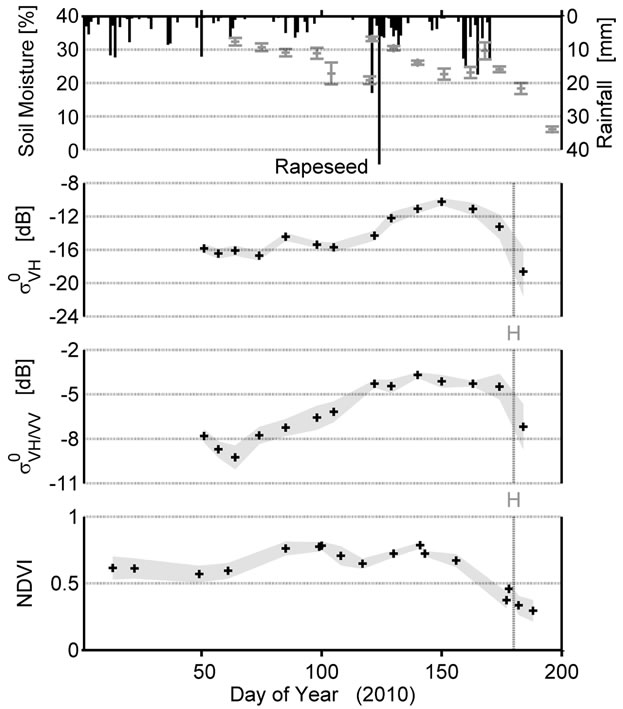 (b)
(b)
Figure 10. Temporal evolution of the backscattering coefficients acquired at C-band over rapeseed fields for the more significant polarization signatures ( and
and ). A time course for the radar signature is presented over one field together with the NDVI, crop height, soil moisture and rainfall events (a); At the landscape scale, the mean and standard deviation are used to delineate satellite signal responses over twelve fields (b). Vertical gray lines and the letter “H” indicate the harvest days.
 (a)
(a)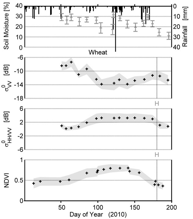 (b)
(b)
Figure 11. Temporal evolution of the backscattering coefficients acquired at C-band over wheat for the more significant polarization signatures ( and
and ). A time course for the radar signature is presented over one field together with the NDVI, crop height, soil moisture and rainfall events (a); At the landscape scale, the mean and standard deviation are used to delineate satellite signal responses over the seventy fields (b). Vertical gray lines and the letter ‘H’ indicate the harvest day.
dynamic of 6 dB is observed in cross-polarization (with only 3 dB in co-polarization). During the first part of the growing season (days 51 to 105), only a few variations, which are all less than 1.5 dB, are observed. At the same time, the NDVI reaches maximal values close to 0.75. The increase in  occurs from days 122 to 150 (corresponding to the period from the end of flowering to seed development) which is more pronounced than at HH polarization (Figure 8); the NDVI shows only few variations, with values close to 0.7. During this period, the complex architecture of the plant is gradually developing (Figure 3). The progressive development of structures without preferred orientations leads to a complex meshing, which explains this increase. All along the rapeseed growth cycle, the cross-polarized signal is not affected by the top soil moisture variations.
The ratio between VH and VV polarizations is also particularly interesting, with a linear increase of approximately 5 dB from days 64 to 140. During sensecence (from day 150 until harvest), the  saturates at values close to −4 dB, while the NDVI decreases until values close to 0.5. No significant effects from the decrease in vegetation water content or top soil moisture variations are observed. The harvest is clearly identifiable, with a decrease of several dB in both single polarization and in the ratio between VH and VV polarizations, at 6 and 3 dB, respectively. This significant decrease in the radar signal is explained by low soil roughness combined with the dry soil conditions that generally occur during harvest. General trends observed over the twelve fields are similar to those observed at a one-field scale. At VH polarization, the signal was very stable in space, with a low standard deviation (with a mean standard deviation value of 0.8 dB) estimated throughout the vegetation cycle. The standard deviation slightly increases with the VH/VV ratio from days 51 to 105, which is associated with heterogeneity in soil conditions (which especially affected the VV polarization, compared to the VH signal). This standard deviation decreases with the augmentation of vegetation from day 121 until harvest in accordance with the reduction of the penetration depth into the crop layer. Considering the NDVI, the maximal variability at landscape scale is observed for the first crop stages, it then decreases when the crop is well established.
Backscattering coefficients extracted at VV polarization over one field of wheat (Figure 11(a)) show a dynamic of approximately 10 dB from the growing period to the harvest. During the crop growth cycle, two interesting periods are observed. The first period occurs during stem elongation, from days 85 to 122, when the vegetation is completely wet. This period implies a linear decrease of  (at the same time, the NDVI reaches maximum values close to 0.8). NDVI and radar signals saturates at the same time. The second period concerns the progressive increase of the
  that occurs during senescence, from day 150 until harvest, when the vegetation is drying. During this period, the decrease of the NDVI is well pronounced and values reaches 0.25 just before harvest. These behaviors are associated with an increase in crop absorption when vegetation is wet, and the opposite effect occurs when vegetation is drying, particularly with the VV polarization state [51]. Over this field, radar signal seems insensitive to the soil moisture variations.
The behavior of  that is observed over 70 fields is associated with a significant standard deviation at the landscape scale (the mean standard deviation is close to 1.4 dB). A discrepancy in crop development, biomass and crop height levels explains the weak trend during senescence (with only a slight increase in the
  compared to Figure 11(a)). Again, the radar signal inflection, from important rainfall events, only appears over all seventy fields. Nevertheless, the effect of soil moisture is less important with vertical polarization (compared to horizontal), backscattering coefficients been dominated by the vegetation component.
The temporal evolution of  has two phases. For the first crop stage, the values are close to 0 dB. They then linearly increase during the stem elongation, then slightly decrease, and finally decrease significantly by 7 dB just before harvest. The same trend is observed over all seventy fields during the growing period with an increase of approximately 4 dB from days 64 to 105. During this period, the NDVI also increases from 0.5 to maximum values. The one monitored field in which a strong radar signal difference is observed before and after harvest cannot be considered as a generality. This difference is locally due to the wheat fell over during a windy period, which induces a high backscatter value with VV polarization and low values of
 . At a landscape scale including over seventy fields, no significant difference is observed before and after harvest, either in the microwave or in the optical domains. Moreover, at this scale, all the satellite signals are saturated at the same times (on day 100) and only NDVI offered significant variation during senescence. The top soil moisture variations do not affect the NDVI nor the
  whatever the study scale.
5.4. Sensitivity to Crop Parameters
In this section, the backscattering coefficients acquired at different frequencies and polarization states are analyzed as a function of two crop parameters: leaf area index (LAI) and crop height (CH). Empirical relationships are estimated for a part of the phenological cycle where maximal sensitivity and accuracy are observed (from the first satellite data to the saturation of the radar signal). Many radar signal combinations are investigated (Tables 3 and 4).
5.4.1. Sensitivity to Leaf Area Index
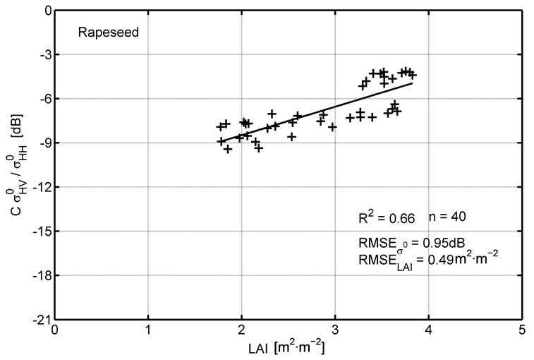
Figure 12 shows two examples of linear relationships between SAR signals and LAI. The best results are obtained by using  and
and  for monitoring the LAI of rapeseed and wheat, respectively. With a coefficient of determination equal to 0.66 (and a rRMSE on LAI of 17%), the ratio of backscattering coefficients acquired at HV and HH polarizations
  provides the LAI of rapeseed with values ranging from 0 to approximately 4 m2∙m−2. Over wheat, the X-band signal shows the highest sensitivity to this vegetation index with approximately 2.6 dB of decrease as the LAI increases by 1 m2∙m−2 (Table 3). By this method, the LAI is estimated with a good confidence interval during growing period (
 , rRMSE = 26%).
Table 3 summarizes the potential of radar multi-frequencies and multi-polarization for monitoring the LAIs of rapeseed and wheat. Coefficients for the linear regressions are given as a and b parameters. The number of sample (n) and statistical indexes (determination coefficient, absolute and relative root mean square errors) are also provided. In addition, the day of the year when the relationship saturates (DOYSAT) and the maximal value of crop parameter reached are also given. For rapeseed, the coefficients of determination (R2) range between 0.37 and 0.66, with associated rRMSE for the LAI ranging from 13% to 33%. With HH polarization, the best results are obtained at Xand L-bands with an rRMSE close to 20%. Furthermore, the overall sensitivities observed with the different frequencies are very close (slopes range from 0.8 to 1 dB by m2∙m−2). The use of coor crosspolarized ratios increase the potential of LAI monitoring by reducing the rRMSE (from 13% to 19%) and increasing the sensitivity (slope close to 2 dB).
For wheat, the coefficients of determination range between 0.10 and 0.64, with an associated rRMSE for the LAI ranging from 26% to 109%. With HH polarization, the best results are obtained at Xand L-bands, as in rapeseed, with an rRMSE equal to 26% and 39%, respectively. The minimum radar signal sensitivity to LAI is
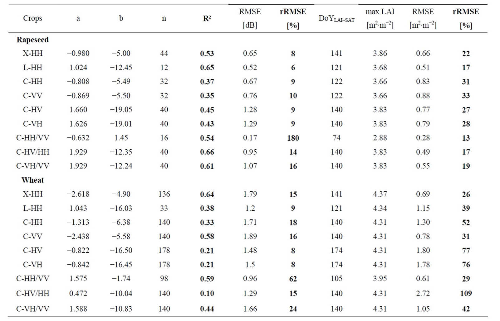
Table 3. Summary of multi-frequency and multi-polarization capabilities for LAI estimation over rapeseed and wheat fields. Slope (a) and offset (b) values of the different linear relationships are given, together with their corresponding statistics for absolute and relative root mean square error and determination coefficient (RMSE, rRMSE and R², respectively). In addition, the day of the year for radar signal saturation (DoYLAI-SAT) and the LAI values reached before saturation are displayed together with the error for the crop parameter.
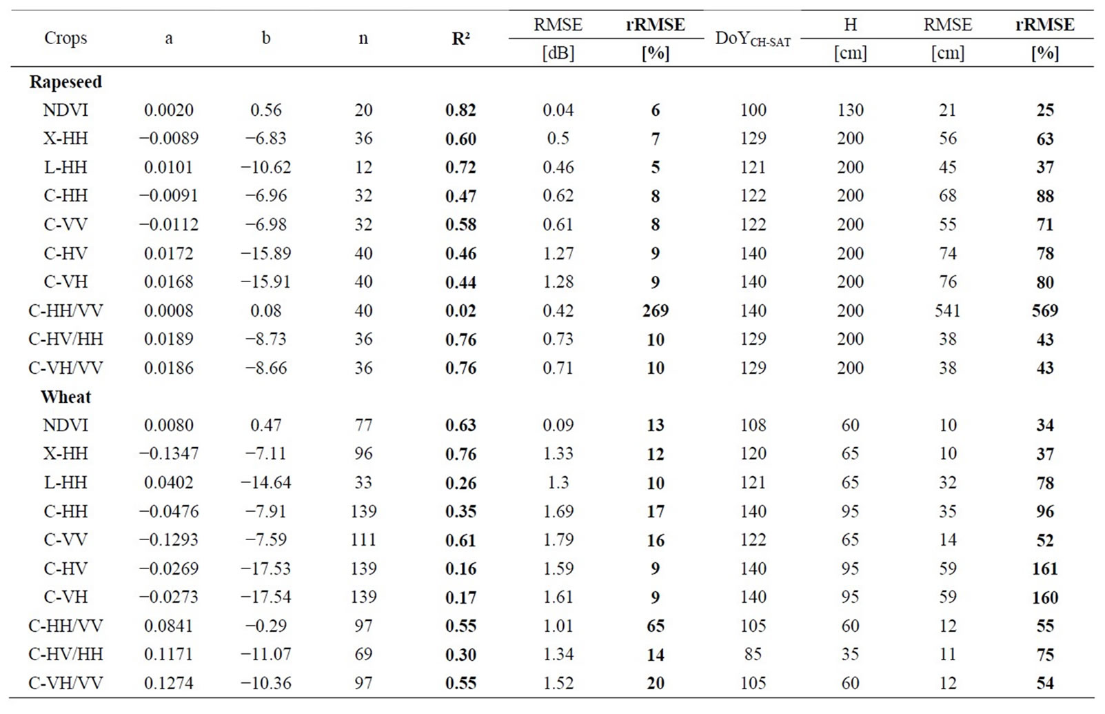
Table 4. Summary of multi-frequency and multi-polarization capabilities for CH estimation over rapeseed and wheat fields. Slope (a) and offset (b) values of the different linear relationships are given, together with their corresponding statistics for the absolute and relative root mean square error and determination coefficients (RMSE, rRMSE and R², respectively). In addition, the day of the year for radar signal saturation (DoYCH-SAT) and the CH values reached before saturation are displayed together with the error of the crop parameter.
 (a)
(a)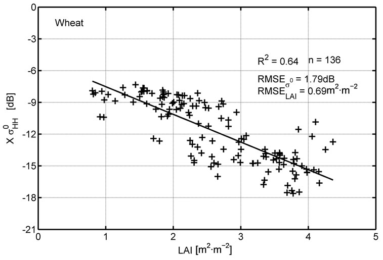 (b)
(b)
Figure 12. Examples of empirical relationships obtained during the growing period between the  and LAI of rapeseed (a) and between the
  and LAI of wheat (b).
observed at L-band, with 1 dB by m2∙m−2, whereas the maximum dynamic is offered by X-band, with 2.6 dB by m2∙m−2. Considering all the radar configurations, three combinations are most relevant for monitoring the LAI of wheat, with an rRMSE close to 30% and R2 superior to 0.58: the  and
and  present similar slopes, and the ratio of co-polarized backscatter offers less sensitivity (1.5 dB by m2∙m−2).
The approach proposed here provides an estimated LAI of wheat and rapeseed until the values are equal to 3.36 and 4.37 m2∙m−2, respectively (by using linear regression functions). Although empirical relationships are not useful over the entire crop cycle, maximal crop parameter values are reached at 3.86 and 4.37 for rapeseed and wheat, respectively. Those results appear promising for the monitoring of winter crops by combining optical and radar data in order to increase temporal satellite sampling and to survey crops even during cloudy conditions.
5.4.2. Sensitivity to Crop Height
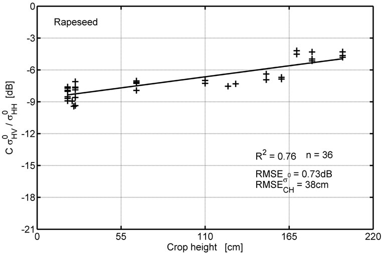
Figure 13 shows two examples of linear relationships that are estimated between the SAR signal and crop height (CH) for rapeseed (Figure 13(a)) and wheat (Figure 13(b)). The best results are obtained by using  and
and  for monitoring the CH of rapeseed and wheat, respectively. The ratio of the C-band backscattering coefficient acquired at HV and HH polarizations
  or
or  allows for the estimation of significant CH (
 , rRMSE = 43%) in rapeseed, for values ranging from 20 cm to 200 cm and a
 (a)
(a)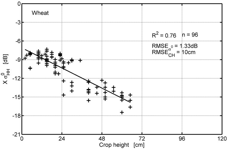 (b)
(b)
Figure 13. Examples of empirical relationships obtained during the growing period between the  and CH of rapeseed (a) and between the
  and CH of wheat (b).
radar sensitivity of approximately 0.02 dB by cm (Table 4). The CH of wheat is also estimated by a linear decreasing function based on the X-band radar signal ( , rRMSE = 37%). For the LAI, the X-band radar represents the highest sensitivity (0.13 dB by cm).
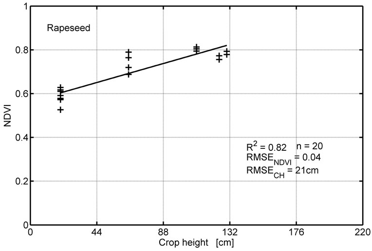
The potential for CH estimation based on optical data is presented in Figure 14. An R2 equal to 0.82 and a relative error of 25% offers higher statistical performance than radar data over the rapeseed (by using a linear regression for being comparable). Nevertheless, a saturation of the NDVI is observed for lower crop height values (near 130 cm instead of 200 cm by using radar data). With an R2 equal to 0.63 and a relative error of 34%, the NDVI over wheat offers a lower statistical performance than those obtained with X-band data for the entire crop cycle. Again, the saturation level is reached with optical data for slightly lower crop height values than for radar signal (60 cm instead of 65 cm).
Table 4 summarizes the capabilities of multi-frequency and multi-polarization potentials for monitoring the CH of rapeseed and wheat. Table 4 includes same parameters as those presented in Table 3. For rapeseed,
 (a)
(a)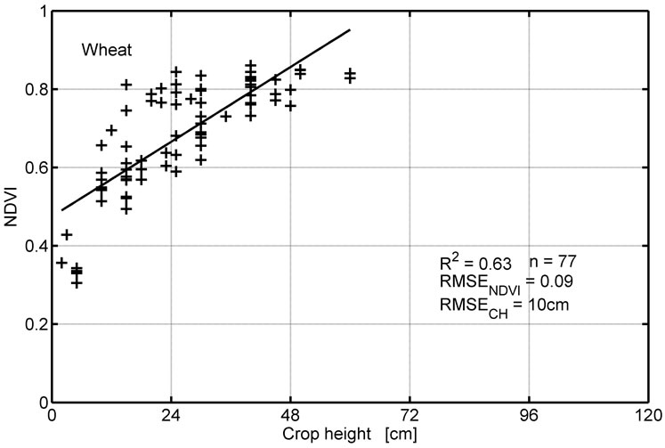 (b)
(b)
Figure 14. Examples of empirical relationships obtained during the growing period between the NDVI and the CH of rapeseed (a) and wheat (b).
the coefficient of determination values are higher, on average, than in the previous section and range from 0.02 to 0.76, with an associated rRMSE in the CH range from 569% to 37%. At HH polarization, the best results are obtained at Xand L-bands with rRMSEs equal to 67% and 37%, respectively. The use of a coor cross-polarized ratio increases the potential of CH monitoring by both increasing the coefficient of determination and the sensitivity ( , slope = 0.02 dB by cm) and reducing the rRMSE (rRMSE = 43%). Regardless of the frequency or polarization of the radar signal, the CH of rapeseed is estimated over the whole range of height values (from 0 cm to 200 cm).
For wheat, the coefficients of determination range between 0.16 and 0.76, with an associated rRMSE ranging from 37% to 161%. At HH polarization, the best results are clearly obtained at X-band (R2 = 0.76), with an rRMSE equal to 37%. Considering all the radar configurations, only three other combinations offer significant relationships , with a coefficient of determination superior to 0.55 and an rRMSE inferior to 55%. Empirical relationships estimated over wheat are not useful over the entire crop cycle (the maximum measured CH reached up to 100 cm). Their validity domain ranges from 0 cm to 65 or 95 cm, depending on the radar frequency and polarization state.
6. Conclusions
This paper investigates the sensitivity of multi-frequency and multi-polarization radar backscatter signatures during the growing seasons of rapeseed and wheat. Time series of satellite images are acquired in 2010 from TerraSAR-X, Radarsat-2 and Alos for radar, and from Formosat-2, Spot-4/5 for optical, in the framework of the MCM’10 experiment. Temporal signatures are first studied after an angular correction (at Xand C-bands) based on the use of satellite optical and SAR data. The sensitivity of satellite signals to crop parameters is then analyzed by considering the leaf area index as derived from optical images and crop heights measured in the fields. Influences of soil conditions (roughness and moisture) are discussed all along the crop cycle.
The angular correction takes advantage of both satellite series that were acquired in optical and microwave domains to select image pairs and maximize the effect of the incidence angles between the closest acquisitions and to reduce the effect of soil conditions changes. The angular normalization of radar signals shows that it is much more important to normalize the radar signal for low NDVI values (<0.4), especially for co-polarized signals acquired at C-band for wheat and rapeseed. The  and
and  show an angular sensitivity that ranges from 0.1 dB.˚−1 (for NDVI close to 0.4) to 0.3 dB.˚−1 over bare soils (with an NDVI close to 0.2). For higher NDVI values (>0.4), the angular normalization is less significant, with a co-polarized radar signal sensitivity less than to 0.05 dB.˚−1. For
  and
and , lower angular sensitivities are observed for low NDVI values (0.08 dB.˚−1 < Ds0 < 0.18 dB.˚−1). For all observed radar configurations, the angular sensitivity is less than to 0.1 dB.˚−1 for NDVI values superior to 0.4.
The times series of optical and angular-normalized radar data show both: the strong complementarities in the multi-sensor approach during the entire crop cycle, and the specific radar behaviors of the two considered crops. According to the rapeseed, contrasting behaviors are observed at the different frequencies. Backscatters acquired with the same polarization (HH), show maximal sensitivity at X-band. At L-band, although the important standard deviation observed at landscape scale, well-marked relationships are estimated with the two crop parameters (LAI and height). Nevertheless, the most suitable results during rapeseed growing cycle are offered by C-band. The cross-polarized backscatters ( or
or ) and ratios taking into account coand cross-polarized backscatters (
 or
or ) show a seasonal dynamic of several dB (~6 dB), during the main part of the crop growth cycle (from first phenological stages to pods development), while the NDVI early saturates. Furthermore, the relationships based on the backscatters ratios offer performances in good agreement for parameter inversion, with R² of 0.66 and 0.76, for LAI and CH respectively.
According to the wheat, similar behaviors are observed at Xand C-bands (affected at landscape scale by the different date of sowing and the various crop developments). The 10 dB of dynamic, observed during the stems elongation, are displayed by both X-band data with HH polarization and C-band with VV polarization. During this period, the NDVI is less sensitive and only increases of 0.2. At the opposite, during the crop senescence, the NDVI decreases with a dynamic of 0.5; the increase in radar signal is less pronounced (from 3 to 5 dB). Crop parameters appear accurately estimated by the shorter wavelength (i.e. X-band) with R² of 0.64 and 0.76 for LAI and CH respectively.
In the future, the results presented in this paper should be tested using data provided by recent and upcoming space missions such as COSMO-SkyMed, Tandem-X/-L, Sentinel-1/-2, Radarsat Constellation, Alos-2…. The interest of new index, combining optical and radar data will be also achieved in the near future. Furthermore, the continuation of such missions will offer the possibility of building the long time series needed to study the ecosystems facing climate change.
7. Acknowledgements
The authors wish to thank the ESA (European Space Agency), DLR (German Space Agency), CSA (Canadian Space Agency), JAXA (Japan Aerospace eXploration Agency), SOAR Project and CNES (Centre National des Etudes Spatiales) for their support, funding and providing satellite images (proposal HYD0611 and SOAR-EU and Categorie-1 ESA projects No. 6843).
REFERENCES
- P. D. Jones, D. H. Lister, T. J. Osborn, C. Harpham, M. Salmon and C. P. Morice, “Hemispheric and Large-Scale Land-Surface Air Temperature Variations: An Extensive Revision and an Update to 2010,” Journal of Geophysical Research, Vol. 117, No. D5, 2012, Article ID: D05127.
- M. H. I. Dore, “Climate Change and Changes in Global Precipitation Patterns: What Do We Know?” Environment International, Vol. 31, No. 8, 2005, pp. 1167-1181. doi:10.1016/j.envint.2005.03.004
- J. E. Olesen and M. Bindi, “Consequences of Climate Change for European Agricultural Productivity, Land Use and Policy,” European Journal of Agronomy, Vol. 16, No. 4, 2002, pp. 239-262. doi:10.1016/S1161-0301(02)00004-7
- P. Falloon and R. Betts, “Climate Impacts on European Agriculture and Water Management in the Context of Adaptation and Mitigation—The Importance of an Integrated Approach,” Science of The Total Environment, Vol. 408, No. 23, 2010, pp. 5667-5687. doi:10.1016/j.scitotenv.2009.05.002
- J. E. Olesen, M. Trnka, K. C. Kersebaum, A. O. Skjelvag, B. Seguin, P. Peltonen-Sainio, F. Rossi, J. Kozyra and F. Micale, “Impacts and Adaptation of European Crop Production Systems to Climate Change,” European Journal of Agronomy, Vol. 34, No. 2, 2011, pp. 96-112. doi:10.1016/j.eja.2010.11.003
- E. M. Hansen and J. Djurhuus, “Nitrate Leaching as Influenced by Soil Tillage and Catch Crop,” Soil and Tillage Research, Vol. 41, No. 3-4, 1997, pp. 203-219. doi:10.1016/S0167-1987(96)01097-5
- P. Béziat, E. Ceschia and G. Dedieu, “Carbon Balance of a Three Crop Succession over Two Cropland Sites in South West France,” Agricultural and Forest Meteorology, Vol. 149, No. 10, 2009, pp. 1628-1645. doi:10.1016/j.agrformet.2009.05.004
- E. Ceschia, P. Béziat, J. F. Dejoux, M. Aubinet, C. Bernhofer, B. Bodson, N. Buchmann, A. Carrara, P. Cellier, P. Di Tommasi, J. A. Elbers, W. Eugster, T. Grünwald, C. M. J. Jacobs, W. W. P. Jans, M. Jones, W. Kutsch, G. Lanigan, E. Magliulo, O. Marloie, E. J. Moors, C. Moureaux, A. Olioso, B. Osborne, M. J. Sanz, M. Saunders, P. Smith, H. Soegaard and M. Wattenbach, “Management Effects on Net Ecosystem Carbon and GHG Budgets at European Crop Sites,” Agriculture, Ecosystems and Environment, Vol. 139, No. 3, 2010, pp. 363- 383. doi:10.1016/j.agee.2010.09.020
- P. R. Ward, K. C. Flower, N. Cordingley, C. Weeks and S. F. Micin, “Soil Water Balance with Cover Crops and Conservation Agriculture in a Mediterranean Climate,” Field Crops Research, Vol. 132, 2012, pp. 33-39. doi:10.1016/j.fcr.2011.10.017
- W. G. M. Bastiaanssen, D. J. Molden and I. W. Makin, “Remote Sensing for Irrigated Agriculture: Examples from Research and Possible Applications,” Agricultural Water Management, Vol. 46, No. 2, 2000, pp. 137-155. doi:10.1016/S0378-3774(00)00080-9
- S. Kalluri, P. Gilruth and R. Bergman, “The Potential of Remote Sensing Data for Decision Makers at the State, Local and Tribal Level: Experiences from NASA’s Synergy Program,” Environmental Science & Policy, Vol. 6, No. 6, 2003, pp. 487-500. doi:10.1016/j.envsci.2003.08.002
- S. K. Seelan, S. Laguette, G. M. Casady and G. A. Seielstad, “Remote Sensing Applications for Precision Agriculture: A Learning Community Approach,” Remote Sensing of Environment, Vol. 88, No. 1-2, 2003, pp. 157-169. doi:10.1016/j.rse.2003.04.007
- F. T. Ulaby, R. K. Moore and A. K. Fung, “Microwave Remote Sensing: Active and Passive, Volume I, Microwave Remote Sensing Fundamentals and Radiometry,” Addison-Wesley, Reading, 1981.
- F. T. Ulaby, R. K. Moore and A. K. Fung, “Microwave Remote Sensing: Active and Passive, Volume III, From Theory to Application,” Artech House, Dedham, 1986.
- F. T. Ulaby, P. P. Batlivala and M. C. Dobson, “Microwave Backscatter Dependence on Surface Roughness, Soil Moisture, and Soil Texture: Part I-Bare Soil,” IEEE Transactions on Geoscience Electronics, Vol. 16, No. 4, 1978, pp. 286-295. doi:10.1109/TGE.1978.294586
- F. T. Ulaby, G. A. Bradley and M. C. Dobson, “Microwave Backscatter Dependence on Surface Roughness, Soil Moisture, and Soil Texture: Part II-Vegetation-Covered Soil,” IEEE Transactions on Geoscience Electronics, Vol. 17, No. 2, 1979, pp. 33-40. doi:10.1109/TGE.1979.294626
- M. C. Dobson and F. Ulaby, “Microwave Backscatter Dependence on Surface Roughness, Soil Moisture, And Soil Texture: Part III-Soil Tension,” IEEE Transactions on Geoscience and Remote Sensing, Vol. GE-19, No. 1, 1981, pp. 51-61. doi:10.1109/TGRS.1981.350328
- S. Le Hegarat-Mascle, M. Zribi, F. Alem, A. Weisse and C. Loumagne, “Soil Moisture Estimation from ERS/SAR Data: Toward an Operational Methodology,” IEEE Transactions on Geoscience and Remote Sensing, Vol. 40, No. 12, 2002, pp. 2647-2658. doi:10.1109/TGRS.2002.806994
- M. Zribi, N. Baghdadi, N. Holah and O. Fafin, “New Methodology for Soil Surface Moisture Estimation and Its Application to ENVISAT-ASAR Multi-Incidence Data Inversion,” Remote Sensing of Environment, Vol. 96, No. 3-4, 2005, pp. 485-496. doi:10.1016/j.rse.2005.04.005
- H. McNairn, A. Merzouki, A. Pacheco and J. Fitzmaurice, “Monitoring Soil Moisture to Support Risk Reduction for the Agriculture Sector Using RADARSAT-2,” IEEE Journal of Selected Topics in Applied Earth Observations and Remote Sensing, Vol. 5, No. 3, 2012, pp. 824-834. doi:10.1109/JSTARS.2012.2192416
- S. C. M. Brown, S. Quegan, K. Morrison, J. C. Bennett, et al., “High-Resolution Measurements of Scattering in Wheat Canopies: Implications for Crop Parameter Retrieval,” ETATS-UNIS: Institute of Electrical and Electronics Engineers, New York, 2003.
- A. Balenzano, F. Mattia, G. Satalino and M. W. J. Davidson, “Dense Temporal Series of Cand L-Band SAR Data for Soil Moisture Retrieval Over Agricultural Crops,” IEEE Journal of Selected Topics in Applied Earth Observations and Remote Sensing, Vol. 4, No. 2, 2011, pp. 439-450. doi:10.1109/JSTARS.2010.2052916
- P. Saich and M. Borgeaud, “Interpreting ERS SAR Signatures of Agricultural Crops in Flevoland, 1993-1996,” IEEE Transactions on Geoscience and Remote Sensing, Vol. 38, No. 2, 2000, pp. 651-657. doi:10.1109/36.841995
- F. Mattia, T. Le Toan, G. Picard, F. I. Posa, A. D’Alessio, C. Notarnicola, A. M. Gatti, M. Rinaldi, G. Satalino and G. Pasquariello, “Multitemporal C-Band Radar Measurements on Wheat Fields,” IEEE Transactions on Geoscience and Remote Sensing, Vol. 41, No. 7, 2003, pp. 1551-1560. doi:10.1109/TGRS.2003.813531
- B. A. M. Bouman and H. W. J. van Kasteren, “GroundBased X-Band (3-cm Wave) Radar Backscattering of Agricultural Crops. II. Wheat, Barley, and Oats; The Impact of Canopy Structure,” Remote Sensing of Environment, Vol. 34, No. 2, 1990, pp. 107-119. doi:10.1016/0034-4257(90)90102-R
- L. Dente, G. Satalino, F. Mattia and M. Rinaldi, “Assimilation of Leaf Area Index Derived from ASAR and MERIS Data into CERES-Wheat Model to Map Wheat Yield,” Remote Sensing of Environment, Vol. 112, No. 4, 2008, pp. 1395-1407. doi:10.1016/j.rse.2007.05.023
- S. Mangiarotti, P. Mazzega, L. Jarlan, E. Mougin, F. Baup and J. Demarty, “Evolutionary Bi-Objective Optimization of a Semi-Arid Vegetation Dynamics Model with NDVI and Backscattering Coefficient Satellite data,” Remote Sensing of Environment, Vol. 112, No. 4, 2008, pp. 1365-1380. doi:10.1016/j.rse.2007.03.030
- R. Hadria, B. Duchemin, F. Baup, T. Le Toan, A. Bouvet, G. Dedieu and M. Le Page, “Combined Use of Optical and Radar Satellite Data for the Detection of Tillage and Irrigation Operations: Case Study in Central Morocco,” Agricultural Water Management, Vol. 96, No. 7, 2009, pp. 1120-1127. doi:10.1016/j.agwat.2009.02.010
- R. Hadria, B. Duchemin, L. Jarlan, G. Dedieu, F. Baup, S. Khabba, A. Olioso and T. Le Toan, “Potentiality of Optical and Radar Satellite Data at High Spatio-Temporal Resolutions for the Monitoring of Irrigated Wheat Crops in Morocco,” International Journal of Applied Earth Observation and Geoinformation, Vol. 12, Suppl. 1, 2010, pp. S32-S37. doi:10.1016/j.jag.2009.09.003
- R. Fieuzal, B. Duchemin, L. Jarlan, M. Zribi, F. Baup, O. Merlin, O. Hagolle and J. Garatuza-Payan, “Combined Use of Optical and Radar Satellite Data for the Monitoring of Irrigation and Soil Moisture of Wheat Crops,” Hydrology and Earth System Sciences, Vol. 15, Special Issue, 2011, pp. 1117-1129. doi:10.5194/hess-15-1117-2011
- M. S. Moran, L. Alonso, J. F. Moreno, M. P. C. Mateo, D. F. de la Cruz and A. Montoro, “A RADARSAT-2 Quad-Polarized Time Series for Monitoring Crop and Soil Conditions in Barrax, Spain,” IEEE Transactions on Geoscience and Remote Sensing, Vol. 50, No. 4, 2012, pp. 1057-1070. doi:10.1109/TGRS.2011.2166080
- M. S. Moran, A. Vidal, D. Troufleau, Y. Inoue and T. A. Mitchell, “Kuand C-Band SAR for Discriminating Agricultural Crop and Soil Conditions,” IEEE Transactions on Geoscience and Remote Sensing, Vol. 36, No. 1, 1998, pp. 265-272. doi:10.1109/36.655335
- K. Dabrowska-Zielinska, Y. Inoue, W. Kowalik and M. Gruszczynska, “Inferring the Effect of Plant and Soil Variables on Cand L-Band SAR Backscatter over Agricultural Fields, Based on Model Analysis,” Advances in Space Research, Vol. 39, No. 1, 2007, pp. 139-148. doi:10.1016/j.asr.2006.02.032
- N. Baghdadi, N. Boyer, P. Todoroff, M. El Hajj and A. Bégué, “Potential of SAR Sensors TerraSAR-X, ASAR/ ENVISAT and PALSAR/ALOS for Monitoring Sugarcane Crops on Reunion Island,” Remote Sensing of Environment, Vol. 113, No. 8, 2009, pp. 1724-1738. doi:10.1016/j.rse.2009.04.005
- X. Jiao, H. McNairn, J. Shang and J. Liu, “The Sensitivity of Multi-Frequency (X, C and L-Band) Radar Backscatter Signatures to Bio-Physical Variables (LAI) over Corn and Soybean Fields,” ISPRS TC VII Symposium—100 Years ISPRS, Vienna, 5-7 July 2010, pp. 317-325.
- F. Baup, R. Fieuzal, C. Marais-Sicre, J. F. Dejoux, V. le Dantec, P. Mordelet, M. Claverie, O. Hagolle, A. Lopes, P. Keravec, E. Ceschia, A. Mialon and R. Kidd, “MCM’10: An Experiment for Satellite Multi-Sensors Crop Monitoring from High to Low Resolution Observations,” 2012 IEEE International Geoscience and Remote Sensing Symposium (IGARSS), Munich, 22-27 July 2012, pp. 4849-4852.
- U. Meier, “Stades Phénologiques des Mono-et Dicotylédones Cultivées,” Centre Fédéral de Recherches Biologiques pour l`Agriculture et les Forêts, 2001. www.agroedieurope.fr/ref/doc/BBCH.pdf
- J.-S. Chern, J. Ling and S.-L. Weng, “Taiwan’s Second Remote Sensing Satellite,” Acta Astronautica, Vol. 63, No. 11-12, 2008, pp. 1305-1311. doi:10.1016/j.actaastro.2008.05.022
- M. Arnaud and M. Leroy, “SPOT 4: A New Generation of SPOT Satellites,” ISPRS Journal of Photogrammetry and Remote Sensing, Vol. 46, No. 4, 1991, pp. 205-215. doi:10.1016/0924-2716(91)90054-Y
- O. Hagolle, G. Dedieu, B. Mougenot, V. Debaecker, B. Duchemin and A. Meygret, “Correction of Aerosol Effects on Multi-Temporal Images Acquired with Constant Viewing Angles: Application to Formosat-2 Images,” Remote Sensing of Environment, Vol. 112, No. 4, 2008, pp. 1689-1701. doi:10.1016/j.rse.2007.08.016
- J. W. Rouse, R. H. Haas, J. A. Schell, D. W. Deering and J. C. Harlan, “Monitoring the Vernal Advancements and Retrogradation of Natural Vegetation,” 1974.
- D. Haboudane, J. R. Miller, E. Pattey, P. J. Zarco-Tejada and I. B. Strachan, “Hyperspectral Vegetation Indices and Novel Algorithms for Predicting Green LAI of Crop Canopies: Modeling and Validation in the Context of Precision Agriculture,” Remote Sensing of Environment, Vol. 90, No. 3, 2004, pp. 337-352. doi:10.1016/j.rse.2003.12.013
- J. Liu, E. Pattey, J. Shang, S. Admiral, G. Jégo, H. McNairn, A. Smith, B. Hu, F. Zhang and J. Freemantle, “Quantifying Crop Biomass Accumulation Using MultiTemporal Optical Remote Sensing Observations,” 30th Canadian Symposium on Remote Sensing, Lethbridge, 22-25 June 2009, 10p.
- H. Breit, T. Fritz, U. Balss, M. Lachaise, A. Niedermeier and M. Vonavka, “TerraSAR-X SAR Processing and Products,” IEEE Transactions on Geoscience and Remote Sensing, Vol. 48, No. 2, 2010, pp. 727-740. doi:10.1109/TGRS.2009.2035497
- L. C. Morena, K. V. James and J. Beck, “An Introduction to the RADARSAT-2 Mission,” Canadian Journal of Remote Sensing, Vol. 30, No. 3, 2004, pp. 221-234. doi:10.5589/m04-004
- A. Rosenqvist, M. Shimada, N. Ito and M. Watanabe, “ALOS PALSAR: A Pathfinder Mission for Global-Scale Monitoring of the Environment,” IEEE Transactions on Geoscience and Remote Sensing, Vol. 45, No. 1, 2007, pp. 3307-3316. doi:10.1109/TGRS.2007.901027
- T. Fritz, M. Eineder, J. Mittermayer, A. Roth, E. Börner and H. Breit, “TerraSAR-X Ground Segment Basic Product Specification Document,” DLR, London, 2008, p. 103.
- NEST, “Next ESA SAR Toolbox,” 2009. http://nest.array.ca/web/nest
- M. Lavalle and T. Wright, “Absolute Radiometric and Polarimetric Calibration of ALOS PALSAR Products,” 2009, p. 18. http://earth.eo.esa.int/pcs/alos/palsar/articles/Calibration_palsar_products_v13.pdf
- H. Skriver, M. T. Svendsen and A. G. Thomsen, “Multitemporal Cand L-Band Polarimetric Signatures of Crops,” IEEE Transactions on Geoscience and Remote Sensing, Vol. 37, No. 5, 1999, pp. 2413-2429. doi:10.1109/36.789639
- G. Cookmartin, P. Saich, S. Quegan, R. Cordey, P. Burgess-Allen and A. Sowter, “Modeling Microwave Interactions with Crops and Comparison with ERS-2 SAR Observations,” IEEE Transactions on Geoscience and Remote Sensing, Vol. 38, No. 2, 2000, pp. 658-670.