Journal of Mathematical Finance
Vol.08 No.01(2018), Article ID:82779,30 pages
10.4236/jmf.2018.81015
Asymptotic Analysis for Spectral Risk Measures Parameterized by Confidence Level
Takashi Kato
Association of Mathematical Finance Laboratory (AMFiL), Tokyo, Japan

Copyright © 2018 by author and Scientific Research Publishing Inc.
This work is licensed under the Creative Commons Attribution International License (CC BY 4.0).
http://creativecommons.org/licenses/by/4.0/


Received: January 21, 2018; Accepted: February 25, 2018; Published: February 28, 2018
ABSTRACT
We study the asymptotic behavior of the difference as , where is a risk measure equipped with a confidence level parameter , and where X and Y are non-negative random variables whose tail probability functions are regularly varying. The case where is the value-at-risk (VaR) at a, is treated in [1] . This paper investigates the case where is a spectral risk measure that converges to the worst-case risk measure as . We give the asymptotic behavior of the difference between the marginal risk contribution and the Euler contribution of Y to the portfolio . Similarly to [1] , our results depend primarily on the relative magnitudes of the thicknesses of the tails of X and Y. Especially, we find that is asymptotically equivalent to the expectation (expected loss) of Y if the tail of Y is sufficiently thinner than that of X. Moreover, we obtain the asymptotic relationship as , where is a constant whose value likewise changes according to the relative magnitudes of the thicknesses of the tails of X and Y. We also conducted a numerical experiment, finding that when the tail of X is sufficiently thicker than that of Y, does not increase monotonically with a and takes a maximum at a confidence level strictly less than 1.
Keywords:
Spectral Risk Measures, Quantitative Risk Management, Asymptotic Analysis, Extreme Value Theory, Euler Contribution

1. Introduction
The purpose of this paper is to investigate the asymptotic behavior of the difference
(1.1)
as , where X and Y are fat-tailed random variables (loss variables) and is a family of risk measures. The case where is an a-percentile value-at-risk (VaR), has been treated in [1] , where it was shown that the asymptotic behavior of drastically changes according to the relative magnitudes of the thicknesses of the tails of X and Y (the definition of the VaR is given in (2.1) in the next section). In this paper, we study a progressive case in which is given as a parameterized spectral risk measure, and we obtain similar results as in [1] . In particular, we find that if X and Y are independent and if the tail of X is sufficiently fatter than that of Y, then converges to the expected value as whenever are spectral risk measures converging to a risk measure of the worst case scenario. That is, whenever
(1.2)
for each loss random variable Z in some sense. Our result does not require any specific form for , implying that this property is robust. Furthermore, assuming some technical conditions for the probability density functions of X and Y, we study the asymptotic behavior of the Euler contribution, defined as
(1.3)
(see Remark 17.1 in [2] ), and show that is asymptotically equivalent to as . Here, is a constant determined according to the relative magnitudes of the thicknesses of the tails of X and Y.
We now briefly review the financial background for this study. In quantitative financial risk management, it is important to capture tail loss events by using adequate risk measures. One of the most standard risk measures is the VaR. The Basel Accords, which provide a set of recommendations for regulations in the banking industry, essentially recommend using VaR as a measure of risk capital for banks. VaRs are indeed simple, useful, and their values are easy to interpret. For instance, a yearly 99.9% VaR calculated as
means that the probability of a risk event with a realized loss larger than
is 0.1%. In other words, an amount  of risk capital is sufficient to prevent a default with 99.9% probability. The meaning of the amount
  is therefore easy to understand. However, VaRs are often criticized for their lack of subadditivity (see, for instance, [3] [4] [5] and [6] ). VaRs do not reflect the risk diversification effect.
The expected shortfall (ES) has been proposed as an alternative risk measure that is coherent (in particular, subadditive) and tractable, with the risk amount at least that of the corresponding VaR. Note that there are various versions of ES, such as the conditional value-at-risk (CVaR), the average value-at-risk (AVaR), the tail conditional expectation (TCE), and the worst conditional expectation (WCE). These are all equivalent under some natural assumptions (see [4] [7] [8] , and [9] ). It should be noted that the Basel Accords have also considered recently the adoption of ESs as a minimal capital requirement, in order to better capture market tail risks (see for instance [10] and [11] ).
A spectral risk measure (SRM) has been proposed as a generalization of ESs, in [3] . SRMs are characterized by a weight function  that represents the significance of each confidence level for the risk manager. SRMs are equivalent to comonotonic law-invariant coherent risk measures (see Remark 1 in the next section).
VaRs and ESs as risk measures depend on a confidence level parameter . We let
  (resp.,
 ) denote the VaR (resp., ES) with confidence level a. When a is close to 1, the values of
  and
and  are increasing without bound as in (1.2). The parameter a corresponds to the risk aversion level of the risk manager. Higher values of a indicate that the risk manager is more risk-averse and evaluates the tail risk as more severe.
In this paper, we consider a family  of SRMs parameterized by the confidence level a. We make a mathematical assumption that intuitively implies situation (1.2) and investigate the asymptotic behaviors of (1.1) and (1.3) as
 , when the tail probability function of X (resp., Y) is regularly varying with index
  (resp.,
 ). Our main theorem asserts that the asymptotic behaviors of (1.1) and (1.3) strongly depend on the relative magnitudes of
  and
and . Note that our results include the case
 , the inclusion of which was discussed as a future task in [1] .
The rest of this paper is organized as follows. In Section 2, we prepare the basic settings and introduce the definitions for SRMs based on confidence level. In Section 3, we give our main results. We numerically verify our results in Section 4. Finally, Section 5 summarizes our studies. Throughout the main part of this paper, we assume that X and Y are independent. The more general case where X and Y are not independent is studied in Appendix 1. All proofs are given in Appendix 2.
2. Preliminaries
Let  be a standard probability space and let
  denote a set of non-negative random variables defined on
 . For each
 , we denote by
  the distribution function of Z and by
  its tail probability function; that is,
  and
and . Moreover, for each
 , we define
 (2.1)
(2.1)
Note that  is exactly the left-continuous version of the generalized inverse function of
 .
.
We now introduce the definition of SRMs.
Definition 1
1) A Borel measurable function  is called an admissible spectrum if
  is right-continuous, non-decreasing, and satisfies
 (2.2)
(2.2)
2) A risk measure  is called an SRM if there is an admissible spectrum
  such that
 , where

Remark 1 SRMs are law-invariant, comonotonic, and coherent risk measures. However, as shown in [12] [13] , and [14] , if  is atomless, then for any law-invariant comonotonic convex risk measure
 , there is a probability measure
  on
on  such that
 (2.3)
(2.3)
for each . This is due to the generalized Kusuoka representation theorem (Theorem 4.93 in [12] ), where
  is the a-percentile expected shortfall of Z:
 (2.4)
(2.4)
Moreover, such a  is always coherent and satisfies the Fatou property [13] . Furthermore, representation (2.3) can also be rewritten as
 , where

Here, it is easy to see that  is non-negative, non-decreasing, right-continuous, and satisfies

meaning that  is an admissible spectrum (see [15] ). Therefore, any law-invariant comonotonic convex (or coherent) risk measure is completely characterized as an SRM. Arguments similar to those above, replacing
  with
with , where
 , can be found in [15] and [16] .
Next, we introduce a family  of SRMs parameterized by the confidence level a.
Definition 2 Let  be a family of admissible spectra and let
 . Then
  is called a set of confidence-level-based spectral risk measures (CLBSRMs) if
 (2.5)
(2.5)
where  is a probability measure on
  defined by
  and
and  is the Dirac measure with unit mass at 1.
Condition (2.5) formally implies (1.2). Indeed, if  is a bounded random variable with a distribution function that is continuous and strictly increasing on
 , where
 , then the function
  is bounded and continuous, so that (2.5) gives

where we recognize . Moreover, we see that
Lemma 1 Relation (2.5) is equivalent to
 (2.6)
(2.6)
We now give some examples of CLBSRMs.
Example 1. Expected Shortfalls
 defined by (2.4) is a typical example of a CLBSRM. The corresponding admissible spectra are given as

It is easy to see that (2.5) does hold. Indeed, for any bounded continuous function f defined on , we see that

due to the bounded convergence theorem. Equivalently, we can also check that  satisfies (2.6).
 is characterized as the smallest law-invariant coherent risk measures that are greater than or equal to
  [14] . Note that if the distribution function of the target random variable Z is continuous, then
  coincides with
 , where

(see [8] for details).
Example 2. Exponential/Power SRMs
An admissible spectrum f corresponding to an SRM  represents the preferences of a risk manager for each quantile of the loss distribution. Therefore, the form taken by f corresponds to the manager’s risk aversion, which is also described in terms of utility functions in classical decision theory. Recently, the relation between expected utility functions and SRMs has been studied, though it has not been entirely resolved. Here we introduce some examples of SRMs based on specific utility functions.
The exponential utility function is a typical example of tractable utility functions

where p denotes the profit-and-loss ( indicating profit) and g characterizes the degree of risk preference. We focus on the case
  so that
  describes a risk-averse utility function. We transform the parameter g into the confidence level
  using
using . Note that the original parameter g can be recovered using the inverse
 . The exponential utility of the loss l with confidence level a is then given as
 . Cotter and Dowd [17] have proposed an SRM
  based on the exponential utility by constructing an admissible spectrum
  for some
 , so that
  satisfies (2.2). Then,
  must be set as
 , giving

Note that the theoretical validity of the above method is still unclear. Other methods to adequately construct SRMs from exponential utility functions have been discussed in [18] [19] , and [20] , but no definite answer has been reached. In particular, it is pointed out in [18] that there exists no general consistency between expected utility theory and SRM-decision making. In any case, we can easily verify that  as defined above satisfies (2.5)-(2.6), which implies that
  is actually a CLBSRM.
Similarly to the above, an SRM  based on the power utility function has been studied in [21] . After changing the risk aversion parameter to the confidence level
  as above,
  is given as

We can also verify that  is a CLBSRM.
We now introduce some notations and definitions used in asymptotic analysis and extreme value theory.
Let f and g be positive functions defined on , where
  and
and . We say that f and g are asymptotically equivalent (denoted as
 ) as
) as  if
if . When
 , we say that f is regularly varying with index
  if it holds that
  for each
 . Moreover, we say that f is ultimately decreasing if f is non-increasing on
  for some
 . For more details, we refer the reader to [22] and [23] .
3. Main Results
Our main purpose is to investigate the property of (1.1) for a CLBSRM  and random variables
  whose distributions are fat-tailed. To consider this case, we assume that
  and
and  are regularly varying functions with indices
  and
and , respectively. That is,
  for each
  and
and
 (3.1)
(3.1)
for some .
.
In [1] , we study the asymptotic property of (1.1) as  when
when . The results display the following five patterns: (i)
 , (ii)
 , (iii)
 , (iv)
 , and (v)
 . In cases (iv) and (v), we consider the difference
  instead of
 , and the results are restated consequences of cases (i) and (ii). Hence, we assume here that
  and focus on cases (i)-(iii) only. We further assume that
 . This assumption guarantees the integrability of X and Y (see, for instance, Proposition A3.8 in [23] ).
Let  be a CLBSRM with a family of admissible spectra
 . Here we assume that
 (3.2)
(3.2)
for each . Then, Lemma A.23 in [12] implies that

for each . This immediately implies that
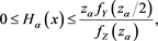
 . Furthermore, by (17.9b) and Proposition 17.2 in [2] , we see that
 (3.3)
(3.3)
where  is given by (1.3) if
  is continuously differentiable in h. Note that inequality (3.3) holds for each
  whenever
  is coherent.
Our main purpose in this section is to investigate in detail the asymptotic behavior of , as well as
  if it is defined, as
 . To clearly state our main results, we establish the following conditions, which are assumed to hold in Section 4 of [1] .
[C1] X and Y are independent.
[C2] There is some  such that
  has a positive, non-increasing
density function  on
on ; that is,
 .
.
[C3] The function  converges to some real number k as
 .
.
Let us adopt the notation
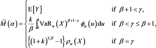 (3.4)
(3.4)
for . Note that
  is finite for each fixed
  (see Corollary 1 in Appendix 2). Our main results are the two following theorems.
Theorem 1 Assuming [C1]-[C3],  as
as .
.
Formally, assertions (i)-(iii) of Theorem 4.1 in [1] are the same as the assumptions of Theorem 1, by setting . That is, we have
  as
as , where
 (3.5)
(3.5)
Theorem 1 justifies the following relation:

Note that condition [C3] is not required for Theorem 1 when . Moreover, when
 , Theorem 1 implies that
  converges to
  as
as . The limit
  does not depend on the forms of
 , so this result is robust. The second main result is as follows.
Theorem 2 Assume [C1] and [C3]. Moreover, assume that
[C4] X and Y have positive, continuous, and ultimately decreasing density functions  and
and , respectively, on
 .
.
Under these assumptions,  as
as , where
  is a positive constant given by
 (3.6)
(3.6)
Theorems 1 and 2 together imply that if X and Y are independent, and if  and
and  have adequate density functions, then
 (3.7)
(3.7)
Note that  is always smaller than or equal to 1, so that (3.7) is consistent with inequality (3.3). In particular, if
 , then the asymptotic equivalence between the marginal risk contribution
  and the Euler contribution
  is justified (see (17.10) in [2] for the definition of marginal risk contributions).
Note that  is always larger than or equal to
  so long as the random vector
  satisfies a suitable technical condition, such as Assumption (S) in [24] . (Here, we modify some conditions of the original version of Assumption (S) to facilitate focusing on non-negative random variables.) Indeed, because
  is a convex risk measure, the function
  is convex. Thus, we get
 (3.8)
(3.8)
where the last equality in the above relation is obtained from (5.12) in [24] ,
 (3.9)
(3.9)
and

due to the dominated convergence theorem. Therefore, if , then

In Section 4, we numerically verify the above relation. Note that we can also verify a version of Assumption (S) under [C4].
Remark 2
1) If  is continuous, then
  has a uniform distribution on
  (see, for instance, Lemma A.21 in [12] ). Therefore,
  with
with  is rewritten as

where  denotes the expectation operator with respect to the probability measure
  defined as
 (3.10)
Note that we have , and so
  represents the risk scenario that attains the maximum in the following robust representation of
 :
:

where  is a set of probability measures on
 . Also note that if
 , then
  is given by

and therefore

Until the end of Remark 2, we assume that  and
and  are continuous.
2) We can relax the independence condition [C1] so that X may weakly depend on Y within the negligible joint tail condition (see Remark A.1 in [1] ). In this case, under some additional assumptions such as [A5] and [A6] in [1] , we can make the same assertion as in Theorem 1, where the value  in the definition (3.4) of
  is replaced by
 . In particular, if
 , then
 (3.11)
Indeed, our proof in Appendix 2 also works by applying Theorem A.1 in [1] instead of Theorem 4.1. Note that we need some additional condition to have that
 (3.12)
(see Proposition 3 in Appendix 2).
3) As mentioned in Appendix A.1 of [1] , we can get another version of Theorem A.1 by switching the roles of  and X and by imposing modified (though somewhat artificial) mathematical conditions such as [A5’] and [A6’] in [1] . In particular, if
 , we see that
 (3.13)
and then (by the same proof as Theorem 1 with (3.13))
 (.14)
(.14)
under some assumptions. Here,  is a probability measure defined by (3.10) with replacing X by
 . If X and Y are independent (with natural assumptions on the density functions), then (3.7) implies that (3.14) is also true. Here, note that the last equality of (3.14) is obtained by (1.3), (3.9), and the dominated convergence theorem. Indeed, we have
 (3.15)
because  is uniformly distributed on
 . In Appendix 1, we will show that under some technical conditions that are more natural than both [A5]-[A6] and [A5’]-[A6’] in [1] , relations (3.11) and (3.14) simultaneously hold in the case
 , even if X and Y are dependent.
Note that if , then

which is known as the component CVaR (also known as the CVaR contribution) and widely used, particularly in the practice of credit portfolio risk management (see for instance [25] [26] , and [27] ).
4. Numerical Analysis
In this section, we numerically investigate the behavior of . Throughout this section, we assume that the distributions of X and Y are given as
  and
and , respectively, with
  and
and , where
  denotes the generalized Pareto distribution whose distribution function is given by
 ,
, . Then,
  and
and  satisfy (3.1) with
  and
and . Note that condition [C3] is satisfied with

(see (5.2) in [1] ). Also note that  and
and  are analytically solved as

We numerically compute , and
, and , where we let
  for brevity. In all calculations, we fix
  and
and . For
. For  and
and , we examine several patterns to study each of the following three cases: 1)
 , 2)
, 2) , and 3)
 .
.
Case 1) 
We set  and
and . Hence,
  and
and , so that
  holds. Figure 1 shows the graphs of
 , and
, and . These values are always larger than
  whenever
 , and they converge to
  for both
  and
and . Indeed,
 (4.1)
(4.1)
holds because ,
,  for each
 . The limit as
  is a consequence of Theorem 1. Moreover, the forms of these graphs are unimodal. That is, the function
  increases on
  and decreases on
  for some
 . Intuitively, the values of
  seem to become large as a increases because a larger a implies a greater risk sensitivity. However, our result implies that the impact of adding loss variable Y into the prior risk profile X is maximized at some
 .
.
Figure 2 shows the relation between  and
and . We see that
  takes a maximum at
 , where
  is a solution to
 (4.2)
(4.2)
Indeed, we have the following result.
Proposition 1 If there is a unique solution  to (4.2), then
 .
.
Note that unlike the case of SRMs,  takes a value smaller than
  if a is small. This is because VaR is not a convex risk measure, so the relation (3.8) is not guaranteed for
 . In particular, we observe that

Figure 1. Graphs of  (blue),
  (orange),
  (green) and
  (black, dashed) with
  and
and . The red solid line shows
 . The horizontal axis corresponds to a.
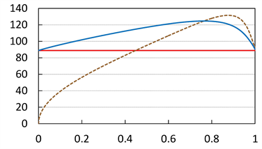
Figure 2. Graphs of  (blue) and
  (brown, dashed) with
  and
and . The red solid line shows
 . The horizontal axis corresponds to a.
 (4.3)
(4.3)
Case 2) 
Figure 3 shows the approximation errors, defined as
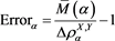 (4.4)
(4.4)
with  (
( ) and
) and  (
( ). We see that
  is close to 0 as
  for each case of
 . Moreover, we numerically verify the assertion of Theorem 2 for
  in Figure 4. We observe that
  converges to
  as
as .
.
By contrast, the convergence speed of  as
as  decreases if the tails of X and Y are less fat-tailed. Figure 5 shows
  with
with  (
( ) and
) and  (
( ). We find that
  decreases as a tends to 1, but the gap between
  and 0 is still large, even in the case
 .
.
Case 3) 
Finally, we look at the case . The results are summarized in Figure 6 and Figure 7. We see that
  approaches 0 as
  for each case of
 . We also confirm that
  converges to
  as
as .
.
Similarly to Case 2), the convergence speed of  decreases as the tails of X and Y become thinner. Figure 8 shows the graph of
  with
with . The approximation error tends to zero as
 , but remains smaller than −20% even when
 .
.
5. Concluding Remarks
In this paper, we have studied the asymptotic behavior of the difference between  and
and  as
as  when
when  is a parameterized SRM satisfying (1.2). We have shown that
  is asymptotically equivalent to
  given by (3.4), whose form changes according to the relative magnitudes
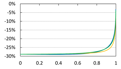
Figure 3. Approximation errors defined by (4.4) with  and
and . Blue line:
 . Orange line:
 . Green line:
 . The horizontal axis corresponds to a.

Figure 4.  (blue) and
  (red). We set
  and
and . The horizontal axis corresponds to a.
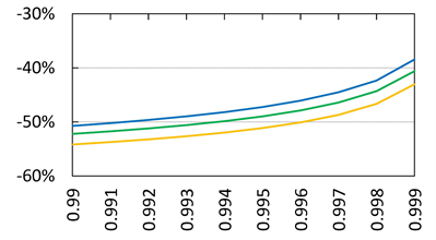
Figure 5. Approximation errors defined by (4.4) with  and
and . Blue line:
 . Orange line:
 . Green line:
 . The horizontal axis corresponds to a.
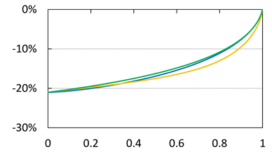
Figure 6. Approximation errors defined by (4.4) with . Blue line:
 . Orange line:
 . Green line:
 . The horizontal axis corresponds to a.
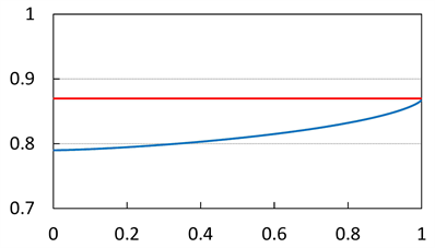
Figure 7.  (blue) and
  (red). We set
 . The horizontal axis corresponds to a.
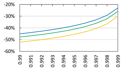
Figure 8. Approximation errors defined by (4.4) with . Blue line:
 . Orange line:
 . Green line:
 . The horizontal axis corresponds to a.
of the thicknesses of the tails of X and Y. In particular, for , we found the convergence
  for general CLBSRMs
 . Moreover, we also found that
  as
as  for a constant
  given by (3.6). This clarifies the asymptotic relation between the marginal risk contribution and the Euler contribution.
Our numerical results in the case  showed that
  is not increasing but is unimodal with respect to a, which implies that the impact of Y in the portfolio
  does not always increase with a. Interestingly, this phenomenon is inconsistent with intuition.
Our results essentially depend on the assumption that X and Y are independent. However, the dependence structure of the loss variables X and Y plays an essential role in financial risk management. The case of dependent X and Y for  has already been studied in Section A.1 of [1] . As mentioned in Remark 2, we have now generalized this result to the case of CLBSRMs. However, we require the somewhat strong assumption that X and Y are not strongly dependent on each other. With the additional analysis in Appendix 1, we will see that our main results still hold for a general dependence structure if
 , but that they are easily violated if
 . In future work, we will continue to study the asymptotic behavior of
  as
as , without the independence condition.
Cite this paper
Kato, T. (2018) Asymptotic Analysis for Spectral Risk Measures Parameterized by Confidence Level. Journal of Mathematical Finance, 8, 197-226. https://doi.org/10.4236/jmf.2018.81015
References
- 1. Kato, T. (2017) Theoretical Sensitivity Analysis for Quantitative Operational Risk Management. International Journal of Theoretical and Applied Finance, 20, 23 p. https://doi.org/10.1007/PL00011399
- 2. Tasche, D. (2008) Capital Allocation to Business Units and Sub-Portfolios: The Euler Principle. In: Resti, A., Ed., Pillar II in the New Basel Accord: The Challenge of Economic Capital, Risk Books, London, 423-453.
- 3. Acerbi, C. (2002) Spectral Measures of Risk: A Coherent Representation of Subjective Risk Aversion. Journal of Banking & Finance, 26, 1505-1518. https://doi.org/10.1016/S0378-4266(02)00281-9
- 4. Acerbi, C. and Tasche, D. (2002) Expected Shortfall: A Natural Coherent Alternative to Value at Risk. Economic Notes, 31, 379-388. https://doi.org/10.1111/1468-0300.00091
- 5. Embrechts, P. (2000) Extreme Value Theory: Potential and Limitations as an Integrated Risk Management Tool, Derivatives Use. Trading & Regulation, 6, 449-456.
- 6. Tasche, D. (2002) Expected Shortfall and Beyond. Journal of Banking & Finance, 26, 1519-1533. https://doi.org/10.1016/S0378-4266(02)00272-8
- 7. Acerbi, C., Nordio, C. and Sirtori, C. (2001) Expected Shortfall as a Tool for Financial Risk Management. Preprint. https://arxiv.org/pdf/cond-mat/0102304.pdf
- 8. Acerbi, C. and Tasche, D. (2002) On the Coherence of Expected Shortfall. Journal of Banking & Finance, 26, 1487-1503. https://doi.org/10.1016/S0378-4266(02)00283-2
- 9. Artzner, P., Delbaen, F., Eber, J.-M. and Heath, D. (1999) Coherent Measures of Risk. Mathematical Finance, 9, 203-228. https://doi.org/10.1111/1467-9965.00068
- 10. Basel Committee on Banking Supervision (2012) Fundamental Review of the Trading Book. Press Release, Bank for International Settlements. http://www.bis.org/publ/bcbs219.pdf
- 11. Basel Committee on Banking Supervision (2016) Minimum Capital Requirements for Market Risk. Press Release, Bank for International Settlements. http://www.bis.org/bcbs/publ/d352.pdf
- 12. Föllmer, H. and Schied, A. (2016) Stochastic Finance: An Introduction in Discrete Time. 4th Edition, De Gruyter. https://doi.org/10.1515/9783110463453
- 13. Jouini, E., Schachermayer, W. and Touzi, N. (2006) Law Invariant Risk Measures Have the Fatou Property, In: Kusuoka, S. and Yamazaki, A., Eds., Advances in Mathematical Economics, 9, 49-71, Springer, Japan. https://doi.org/10.1007/4-431-34342-3_4
- 14. Kusuoka, S. (2001) On Law-Invariant Coherent Risk Measures. In: Kusuoka, S. and Maruyama, T., Eds., Advances in Mathematical Economics, 3, 83-95, Springer, Japan. https://doi.org/10.1007/978-4-431-67891-5_4
- 15. Shapiro, S. (2013) On Kusuoka Representation of Law Invariant Risk Measures. Mathematics of Operations Research, 38, 142-152. https://doi.org/10.1287/moor.1120.0563
- 16. Pflug, G.Ch. and Römisch, W. (2007) Modeling, Measuring and Managing Risk. World Scientific Publishing Co., London. https://doi.org/10.1142/6478
- 17. Cotter, J. and Dowd, K. (2006) Extreme Spectral Risk Measures: An Application to Futures Clearinghouse Margin Requirements. Journal of Banking & Finance, 30, 3469-3485. https://doi.org/10.1016/j.jbankfin.2006.01.008
- 18. Brandtner, M. and Kürsten, W. (2017) Consistent Modeling of Risk Averse Behavior with Spectral Risk Measures: Wächter/Mazzoni Revisited. European Journal of Operational Research, 259, 394-399. https://doi.org/10.1016/j.jbankfin.2006.01.008
- 19. Sriboonchitta, S., Nguyen, H.T. and Kreinovich, V. (2010) How to Relate Spectral Risk Measures and Utilities. International Journal of Intelligent Technologies and Applied Statistics, 3, 141-158. https://doi.org/10.6148/IJITAS.2010.0302.03
- 20. Wächter, H.P. and Mazzoni, T. (2013) Consistent Modeling of Risk Averse Behavior with Spectral Risk Measures. European Journal of Operational Research, 229, 487-495. https://doi.org/10.1016/j.ejor.2013.03.001
- 21. Dowd, K., Cotter, J. and Sorwar, G. (2008) Spectral Risk Measures: Properties and Limitations. Journal of Financial Services Research, 34, 61-75. https://doi.org/10.1007/s10693-008-0035-6
- 22. Bingham, N.H., Goldie, C.M. and Teugels, J.L. (1989) Regular Variation. Cambridge University Press, Cambridge.
- 23. Embrechts, P., Klüppelberg, C. and Mikosch, T. (1997) Modelling Extremal Events, Springer, Berlin. https://doi.org/10.1007/978-3-642-33483-2
- 24. Tasche, D. (2000) Risk Contributions and Performance Measurement, Working Paper. https://pdfs.semanticscholar.org/2659/60513755b26ada0b4fb688460e8334a409dd.pdf
- 25. Andersson, F., Mausser, H., Rosen, D. and Uryasev, S. (2001) Credit Risk Optimization with Conditional Value-at-Risk Criterion. Mathematical Programming Series B, 89, 273-291. https://doi.org/10.1007/PL00011399
- 26. Kalkbrener, M., Kennedy, A. and Popp, M. (2007) Efficient Calculation of Expected Shortfall Contributions in Large Credit Portfolios. Journal of Computational Finance, 11, 1-43. https://doi.org/10.21314/JCF.2007.162
- 27. Puzanova, N. and Düllmann, K. (2013) Systemic Risk Contributions: A Credit Portfolio Approach. Journal of Banking & Finance, 37, 1243-1257. https://doi.org/10.1016/j.jbankfin.2012.11.017
- 28. McNeil, A.J., Frey, R. and Embrechts, P. (2005) Quantitative Risk Management. Princeton University Press, Princeton.
- 29. Bingham, N.H., Goldie, C.M. and Omey, E. (2006) Regularly Varying Probability Densities, Publications de l’Institut Mathematique, 80, 47-57. https://doi.org/10.2298/PIM0694047B
Appendix 1. A Short Consideration of the Dependent Case
Here, we briefly investigate the asymptotic behavior of  as
as  when X and Y are not independent. Throughout this section, we assume that
 ,
,  , and
, and  are continuous. With this, (3.8) is rewritten as
 . Combining this result with (3.3), we have
 (A.1)
(A.1)
Note that (A.1) holds for general SRM  whenever (3.9) holds.
1.1. Comonotonic Case
We consider the case where X and Y are comonotone. In other words, they are perfectly positively dependent (see Definition 4.82 of [12] and Definition 5.15 in [28] ). In this case, the following proposition is straightforwardly shown.
Proposition 2 If X and Y are comonotone, then
 (A.2)
(A.2)
This proposition implies that when , the asymptotic relations (3.11) and (3.14) still hold, even if X and Y are strongly correlated, but that the assertions of Theorems 1 and 2 do not necessarily hold when
 .
.
1.2. Additional Numerical Analysis
Similarly to Section 4, we assume that  and
and  with
with ,
, . To describe the dependence between X and Y, we introduce a copula. By Sklar’s theorem, we see that the joint distribution function
  of the random vector
  is represented by

for a copula , which is a distribution function with uniform marginals. Here, we examine the following three copulas:
1) The Gaussian copula ,
,  ,
,
2) The Gumbel copula ,
,  ,
,
3) The countermonotonic copula ,
,
where  is the distribution function of the standard
normal distribution (for more details on the copulas, see, for instance, Chapter 5 of [28] ). The parameters  in (a) and
  in (b) describe the strength of the dependence between X and Y. We always set
  and
and  in this section. If
 , then X and Y are perfectly negatively dependent. In particular, in that case, X and Y are represented as
  and
and , where U is a random variable with uniform distribution on
 .
.
Figure A1 summarizes the results with  and
and . We compare the values of
  (with
(with ) and
) and . We find that all these values converge to the same value, which is not equal to
 , by letting
 . Note that when X and Y are countermonotonic, they converge to zero as
 , so (3.12) does not hold in this case.
Figure A2 shows the graphs of the relative errors defined by (4.4) with  when we set
  and
and . We find that
  does not converge to zero as
 . Similar phenomena are observed in Figure A3 with the settings
 . Therefore, the assertion of Theorem 1 does not hold when
  if X and Y are correlated.
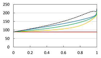


Figure A1. Graphs of  (blue),
  (orange),
  (green) and
  (black, dashed) with
  and
and . The red solid line shows
 . The horizontal axis corresponds to a. Top:
  with
with . Center:
  with
with . Bottom:
 .
.
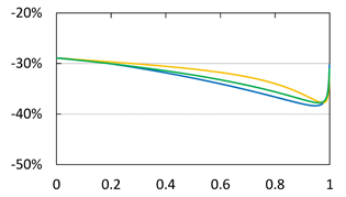
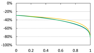

Figure A2. Approximation errors defined by (4.4) with  and
and . Blue line:
 . Orange line:
 . Green line:
 . The horizontal axis corresponds to a. Top:
  with
with . Center:
  with
with . Bottom:
 .
.
Note that the above findings are consistent with the comonotonic case (Proposition 2).
1.3. Theoretical Result in the Case 
We describe the following conditions.
[C5] For each ,
,  has a positive, non-increasing density function
  on
on , where
  is the conditional distribution function of X given
 . Moreover,
  is continuous in
  and y.
[C6] There is a  such that
  is uniformly regularly varying with index
  in the following sense:
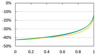
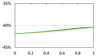
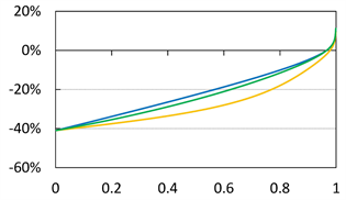
Figure A3. Approximation errors defined by (4.4) with . Blue line:
 . Orange line:
 . Green line:
 . The horizontal axis corresponds to a. Top:
  with
with . Center:
  with
with . Bottom:
 .
.
 (A.3)
(A.3)
for each . Moreover,
  is ultimately decreasing.
[C7] It holds that
 (A.4)
(A.4)
for some .
.
Conditions [C5]-[C7] strongly correspond to conditions [A5]-[A6] in [1] . It should be noted that the index parameter  is assumed to be equal to
  in condition [A6] in [1] , but that this equality is not required to obtain our results. Note also that
  may be different from
 . Indeed, we can verify, at least numerically, that for each
 , the function
  is regularly varying with index
  (resp.,
 ) if we adopt
  (resp.,
 ) as a copula for the random vector
  whose marginal distributions are given by the generalized Pareto distribution.
Using a similar argument as in the proof of the uniform convergence theorem (Theorem 1.2.1 in [22] ), together with the continuity of  in y, we get from (A.3) that
 (A.5)
(A.5)
for each compact set .
.
We now introduce the following result.
Theorem 3 Assume [C5]-[C7] and (3.12). If , it holds that

This theorem claims that both (3.11) and (3.14) are true under some conditions, even when X and Y are dependent.
Appendix 2. Proofs
\Proof of Lemma 1. Assume (2.5). Fix any . Then, (2.5) implies that
 (B.1)
(B.1)
Because  is non-decreasing and non-negative, we see that
 (B.2)
(B.2)
Combining (B.1) with (B.2), we have .
.
Conversely, if we assume (2.6), then Prokhorov’s theorem implies that for
each increasing sequence  with
with  there is a further subsequence
  and a probability measure
  on
on  such that
weakly converges to  as
as . Then, for each
 , we see that

This immediately leads us to , hence
 . We therefore arrive at (2.5).
Proof of Proposition 1. Let . We observe that

where . By (4.1), (4.3), and Theorem 1, we see that g is continuous on
 ,
,  and
and . Moreover, by the assumption, it holds that
  and
and  for all
 . Together, these imply that g is positive on
  and negative on
 , and that
  has the same pattern. Therefore,
  takes a maximum at
 .
.
Proof of Proposition 2. Because  is comonotonic, we obviously have

Here, we see that  and
and  for some random variable U with uniform distribution on
  (see Lemmas 4.89-4.90 in [12] and their proofs). Then we have

and thus

Similarly, because , we have

and , which completes the proof.
2.1. Proof of Theorem 1
We first state some propositions and prove them. For this, let  be given as (3.5). Note again that
  defined in (3.4) satisfies

Proposition 3 .
.
Proof. If , we see that
  because Y is non-negative and
  is positive. If
 , we observe

where  is a real number satisfying
 . The existence of such an
  can be proven using Propositions 1.5.1 and 1.5.15 in [22] . Similarly, if
 , we have

Proposition 4 .
.
Proof. If , the assertion is obvious from the assumption
 . If
. If , we see that

because of . If
. If , we have

Corollary 1 ,
, .
.
Proof. This follows from (3.2) and Proposition 4.
Proof of Theorem 1. Let ,
, . Note that
 (B.3)
(B.3)
by virtue of Theorem 4.1(i)-(iii) in [1] . Moreover, (B.3) immediately implies
 (B.4)
(B.4)
Furthermore, it holds that
 (B.5)
(B.5)
hence  is integrable. The integrability of
  is guaranteed by Proposition 4.
Temporarily fix any . From (2.6) and (B.5), we easily see that
 (B.6)
(B.6)
Similarly, we have
 (B.7)
(B.7)
Additionally, we have
 (B.8)
(B.8)
where . Using (B.7) and Proposition 3, we obtain
 (B.9)
(B.9)
By (B.8) and (B.9), we have

Combining this with (B.6) and Proposition 3, we arrive at

Because  is arbitrary, we obtain the desired assertion by (B.4).
2.2. Proof of Theorem 2
Let  for brevity. We see that Z has a density function

Lemma 2  is positive and continuous on
 . Moreover,
  is regularly varying with index
  and it holds that
 (B.10)
Proof. Continuity and positivity are obvious. By [C4] and Theorem 1.1 in [29] , we see that ,
,  and that
  is regularly varying with index
 . The last assertion is obtained by Proposition 1.5.10 in [22] .
Let  be the conditional distribution function of Y given
 . Then we have
 (B.11)
Proposition 5 It holds that

Proof. For each , a straightforward calculation gives

which implies our assertion.
Note that (B.11) and Proposition 5 lead to
 (B.12)
Proposition 6 If , then

Proof. Let
 (B.13)
 (B.14)
 (B.15)
Then, we see that
 (B.16)
Therefore, we need to show that
 (B.17)
First, we show that
 (B.18)
Using (B.10), Lemmas A.1 and A.3 in [1] , and Proposition A3.8 in [23] , we obtain

Furthermore, we observe that
 (B.19)
and that the function  is regulary varying with index
 . Thus, we obtain

Now, (B.18) is obvious.
Next, we observe that

Because  and
and  are convergent (as
 ), they are bounded. Thus, we have
 (B.20)
for some . By (B.18) and (B.20), we can apply the dominated convergence theorem to obtain (B.17).
Proposition 7 If , then

Proof. Let ,
,  , and
, and  be the same as in (B.13)-(B.15). First, we have
 ,
,  by the same argument as in the proof of Proposition 6. Next, for each
 , we see that

due to [C3], (B.10), Proposition A3.8 in [23] , Proposition 3.1(i) in [1] , and Lemmas A.1 and A.3 in [1] . Moreover, we have (B.19), and the right-hand side of this inequality converges to  as
as , and so it is bounded. Therefore, we apply the dominated convergence theorem to obtain
 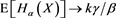 as
as . We complete the proof by combining these with (B.16).
Proposition 8 If , we have

Proof. Let ,
,  and
and  be set as earlier. Similarly to the proof of Propositions 6 and 7, we get
 ,
, . This implies that
 ,
,  , where
 . Therefore, it suffices to show that
  as
as , which is easy to see by using similar calculations as in the proof of Proposition 7 and by using Proposition 3.1(i) in [1] .
Proposition 9 If , then

Proof. Similarly to the proof of Proposition 8, we need to show only that
 (B.21)
where . Note that Lemmas A.1 and A.2 in [1] imply
 ,
,  and
and ,
, . Therefore, for each
 , we observe

by [C3], (B.10), Proposition A3.8 in [23] , and Lemma A.3 in [1] . Moreover, we have

and thus we obtain (B.21) by applying the dominated convergence theorem.
Proof of Theorem 2. We can verify that the random vector  satisfies (a version of) Assumption (S) in [24] by using a standard argument. Therefore, (3.9) is true from (5.13) in [24] . Additionally, using Propositions 6-9, we see that for each
 , there is an
  such that
 (B.22)
where we denote . Moreover, it is easy to see that
  and
and  are bounded on
 . Therefore, combining (3.9), (3.15), and (B.22), we get

where , which is positive due to Proposition 3. Because
 is arbitrary, we obtain the desired assertion.
2.3. Proof of Theorem 3
First, note that condition [C5] immediately implies [C2] with  and
and

Second, note that by [C6], Proposition 3.1(i) in [1] (see also Remark 3.2 therein) and Proposition A3.8 in [23] , we have (B.10) and
 (B.23)
To prove Theorem 3, we give the following three propositions.
Proposition 10  is continuously differentiable in
  and it holds that

Proposition 10 is obtained by an argument similar to the proof of Lemma 5.3 in [24] , using the implicit function theorem.
Proposition 11 The function  is regularly varying with index
 .
.
Proof. Fix any . We observe that

and therefore, using [C5], we arrive at

Proposition 12 .
.
Proof. Fix any . Then we have

where we denote  and
and


By [C7] and the Chebyshev inequality, we get
 (B.24)
for some . Because Proposition 11 tells us that
  is regularly varying with index
 , the right-hand side of (B.24) converges to zero as
  (see Proposition 1.5.1 in [22] ).
Moreover, we see that

Here, we observe that
for each . Note that if
  (resp.,
 ), we have
  (resp.,
 ). Moreover, by (B.23),
  converges to 1 as
 , and so it is bounded. Therefore, we get

for some .
.
Now we arrive at

by using (A.5) and (B.23). Because  is arbitrary, we obtain the desired assertion.
Proof of Theorem 3. First, note that Proposition 10 guarantees that

where  and
and .
.
Then, fix any . By Propositions 11-12 and Lemma A.3 in [1] , we see that

Thus, there is an  such that

Therefore, we have

by virtue of (3.12). Because  is arbitrary, we get that
 ,
, . Combining this result with (A.1), we obtain the desired assertion.