Received 5 December 2015; accepted 24 April 2016; published 27 April 2016

ABSTRACT

In the present paper as estimation of an unknown probability density of the spline-estimation is constructed, necessity and sufficiency conditions of strong consistency of the spline-estimation are given.

Keywords:

Strong Consistency, Spline-Estimation, Probability Density in Uniform Metric, Uniform Metric, Soatov, Muminov, Tashkent University, Institute of Mathematics

1. Introduction

We assume that on the interval, , a < b. The following mesh

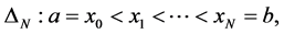(1)

is given, where N is a natural number. Let P_k be the set of polynomials of degree ≤ k and С_k[a, b] be the set of continuous on the [a, b] functions having continuous derivative of order k,. In the book of Stechkin and Subbotin [1] the following is given.

Definition. The function is called by interpolation cubic spline with respect to the mesh (1) for the function F(x), if:

a),

b)

c)

Here

The points are called by the nodes of the spline.

Later on for convenience we let and the obtained results will remain valid for any finite interval [a, b].

Let be independent identical distributed random variables with unknown density distribution f(x) concentrated and continuous on the interval [0, 1], and S_N(x) be cubic spline interpolating the values y_k = F_n(x_k) in the points x_k = kh, , N=N_(n) with “boundary conditions”

Here F_n(x) is the empirical function of the distribution of the sample, and,

as, and are given real numbers. Concrete choice of these numbers depends on the considered problem.

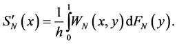
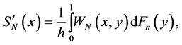
As estimation of an unknown probability density we take the statistics.

In the present work as estimation of the unknown density f(x) we take the statistics defined as in Theorem 1 and in Theorem 2 as well.

It is clear that, in Theorems 1 and 2 spline estimations are constructed with different boundary conditions.

Theorem 3 is devoted to asymptotic unbiasedness of the spline estimation. Also for completeness of the results the dispersion and the covariance of the spline-estimation are given.

In the main Theorem 4 necessity and sufficiency conditions for strong consistency of the spline-estimation are given.

Similar result for the Persen-Rozenblatt estimation is obtained in the book of Nadaraya (1983) [2] .

More detailed review on spline estimation is given in works of Wegman, Wright [3] , Muminov [4] .

2. Auxiliary Results

Using the results of the work Lii [5] the following theorems are easily proved.

2.1. Theorem 1

Let F_n(x) be empirical function of the distribution constructed by simple sample and S_N(x) be cubic spline interpolating the values F_n(x_k) in the nodes of the mesh (1). If we choose the boundary conditions for S_N(x) in the form

then the derivative of the spline function is defined by the equality

Here, for, 0

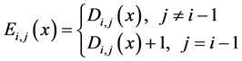
and

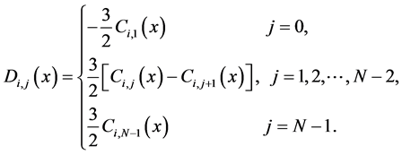
C_i,j(x) are defined by the following relations:

, (2)

where

, for the other i and j.

2.2. Theorem 2

Let F_n(x) be empirical function of the distribution constructed by simple sample and S_N(x) be cubic spline interpolating the values F_n(x_k). in the mesh (1). If we choose the boundary conditions for S_N(x) in the form

Then the derivative of the spline function is defined by the equality

where, for, ,

,

, ,

, ,

, ,

,

and C_i,j are defined by formula (2).

We introduce the following denotations:

is the simple sample from the general population

;

is empirical function of distribution of the sample;

is the empirical process;

is the sequence of wiener processes;

is the brownian bridge.

We give the auxiliary lemmas.

2.3. Lemma 1 [6]

There exists a probability space (Ω, F, P).

On which it can be defined version and the sequence of Brownian bridges B_n(t) such that for all x > 0

where a = 3.26, b = 4.86, с = 2.70.

2.4. Lemma 2 [7]

Let be modulus of continuity of the brownian bridge B_n(t),

and. Then with probability 1 does not exceed the quantity.

Here is the random variable which is not less than 1 almost everywhere and.

3. Main Results and Proofs

The following theorem characterizes the asymptotic behavior of the bias, the covariance and the dispersion of the spline estimation.

3.1. Theorem 3

Let be the spline estimation.

1) If and are defined as in Theorem 2, then for

.

2) If and are defined as in Theorem 1, then

where 0 < x < 1,

[y] is the integer part of the number y.

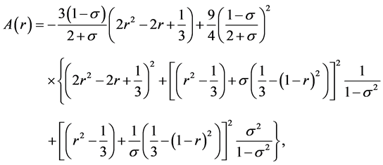
3) Suppose, , , d = i ? j, and, then for

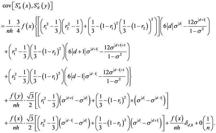
Proof. By virtue of, Theorems 9, 11, 12 from Stechkin and Subbotin [1] and Theorems 1 from Lii [5] follows the first statement of Theorem 3. The second and the third statement of Theorem 3 are proved in Lii [5] .

3.2. Theorem 4

Suppose as. Then in order with probability 1

it is necessary and sufficient that the function g(x) is the density of the distribution F(x) concentrated and continuous on the interval [0,1] with respect to Lebesgue measure.

Proof. Sufficiency. It is clear that

(3)

where

First we estimate the term in the right hand part of (3). We have

(4)

From Lemma 1 it follows that with probability 1 for

(5)

If we denote the modulus of continuity by then from

Lemma 2

(6)

where

with probability and

This, combining (3)-(6) and using Theorem 3 we get the sufficiency condition of Theorem 4.

Necessity. Let with probability 1

Hence, from continuity of it follows continuity of g(x) on the interval [0, 1].

Therefore, the sequence random variables

are uniformly integrable. Therefore according to Theorem 5 from Shiryaev [8] and the inequalities

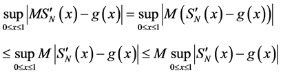
it follows that for

(7)

By virtue of (7) it is easy to see that the sequence of functions

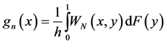
uniformly converges to some continuous function g₀(x), i.e. for

(8)

We show now continuity of F(x) on the interval [0, 1].

We assume the inverse that there exists a point x₀, such that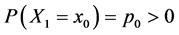. Then by virtue of (8) and

it follows continuity of F(x) on the interval [0, 1].

By (8) for all

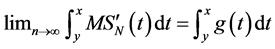(9)

(10)

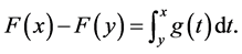
From another side, according to Theorem 11 from Stechkin and Subbotin (1976)

(11)

By virtue of (9)-(11)

Theorem 4 is proved.

Cite this paper

Mukhammadjon S. Muminov,Khaliq S. Soatov, (2016) Strong Consistency of the Spline-Estimation of Probabilities Density in Uniform Metric. Open Journal of Statistics,06,373-379. doi: 10.4236/ojs.2016.62032

References

- 1. Stechkin, S.B. and Subbotin, Y.N. (1976) Splines in Computational Mathematics. Moscow, Nauka, 272 p.
- 2. Nadaraya, E.A. (1983) Nonparametric Estimation of Probability Density and Regression Curve. Tbilisi University, Tbilisi, 195 p.
- 3. Wegman, E.J. and Wright, I.W. (1983) Splinesin Statistics. Journal of the American Statistical Association, 78, 351-365.
http://dx.doi.org/10.1080/01621459.1983.10477977 - 4. Muminov, M.S. (2010) On Appoximation of the Probability of the Lagre Outlier of Nonstationary Gauss Process. Siberian Mathematical Journal, 51, 175-195.
http://dx.doi.org/10.1007/s11202-010-0015-6 - 5. Lii, K.S. (1978) A Global Measure of a Spline Density Estimate. Annals of Statistics, 6, 1138-1148.
http://dx.doi.org/10.1214/aos/1176344316 - 6. Rio, E. (1994) Local Invariance Principles and Application to Density Estimation. Probability Theory and Related Fields, 98, 21-26.
http://dx.doi.org/10.1007/BF01311347 - 7. Garsia, F. (1970) Continuity Properties of Gaussian Processer with Multidimensional Time Parameter. Proceedings of the Sixth Berkeley Symposium on Mathematical Statistics and Probability, 369-374.
- 8. Shiryaev, A.N. (1982) Probability. Moscow, Nauka, 576 p.