Paper Menu >>
Journal Menu >>
 Int. J. Communications, Network and System Sciences, 2010, 3, 321–329 doi:10.4236/ijcns.2010.33041 blished Online March 2010 (http://www.SciRP.org/journal/ijcns/). Copyright © 2010 SciRes. IJCNS Pu Time Domain Signal Analysis Using Wavelet Packet Decomposition Approach M. Y. Gokhale1, Daljeet Kaur Khanduja2 1Professor and Head of Department of Mathematics, Maharashtra Institute of Technology, Pune, India 2Assistant Professor Department of Mathematics, Sinhgad Academy of Engineering, Pune, India Email: dkdkhalsa@gmail.com Received November 11, 2009; revised December 17, 2009; accepted January 22, 2010 Abstract This paper explains a study conducted based on wavelet packet transform techniques. In this paper the key idea underlying the construction of wavelet packet analysis (WPA) with various wavelet basis sets is elabo- rated. Since wavelet packet decomposition can provide more precise frequency resolution than wavelet de- composition the implementation of one dimensional wavelet packet transform and their usefulness in time signal analysis and synthesis is illustrated. A mother or basis wavelet is first chosen for five wavelet filter families such as Haar, Daubechies (Db4), Coiflet, Symlet and dmey. The signal is then decomposed to a set of scaled and translated versions of the mother wavelet also known as time and frequency parameters. Analysis and synthesis of the time signal is performed around 8 seconds to 25 seconds. This was conducted to determine the effect of the choice of mother wavelet on the time signals. Results are also prepared for the comparison of the signal at each decomposition level. The physical changes that are occurred during each decomposition level can be observed from the results. The results show that wavelet filter with WPA are use- ful for analysis and synthesis purpose. In terms of signal quality and the time required for the analysis and synthesis, the Haar wavelet has been seen to be the best mother wavelet. This is taken from the analysis of the signal to noise ratio (SNR) value which is around 300 dB to 315 dB for the four decomposition levels. Keywords: WPA, Wavelet Packet Decomposition (WPD), SNR, Haar 1. Introduction Over the last decade much work has been done in apply- ing time frequency transforms to the problem of signal representation and classification. Signals possessing non-stationary character are not well suited for detection and classification by traditional Fourier methods. It has been shown that wavelets can approximate time varying non-stationary signals in a better way than the Fourier transform representing the signal on both time and fre- quency domains [1]. Hence they can easily detect local features in a signal. Furthermore, wavelet decomposition allows analyzing a signal at different resolution levels. The discrete wavelet transform (DWT) provides a very efficient representation for a broad range of real-world signals. This property has been exploited to develop powerful signal de-noising and estimation methods [2] and extremely low-bit-rate compression algorithms [3].The discrete wavelet transform (DWT) is usually imple- mented using an octave-band tree structure. This is ac- complished by dividing each sequence into a component containing its approximated version (low-frequency part) and a component with the residual details (high-frequ- ency part) and then iterating this procedure at each stage only on the low-pass branch of the tree [4,5]. The main drawback of the octave-band tree structure is that it does not provide a good approximation of the critical subband decomposition [6]. An alternate means of analysis is sought, so that valuable time-frequency information is not lost. The Wavelet Packet Transform (WPT) is one such time frequency analysis tools. It is a transform that brings the signal into a domain that contains both time and frequency information (Wickerhauser, 1991). Thus, analy- sis of the signal can be done simultaneously in frequency and time. The most basic way to do time frequency analysis is by making FFT analysis in short windows. That has the drawback that the window needs to be short to find out fast changes in the signal and long to determine low frequency components. The wavelet packet trans- form (WPT) offers a great deal of freedom in dealing  M. Y. GOKHALE ET AL. 322 with different types of transient signals. Indeed the de- velopment of the wavelet transform (WT) [7–9] and wavelet packets [10–12] has sparked considerable activ- ity in signal representation and in transient and non sta- tionary signal analysis.[13–15]. Wavelet packet decomposition (WPD) (sometimes known as just wavelet packets) is a wavelet transform where the signal is passed through more filters than the DWT. Wavelet packets are the particular linear combina- tion of wavelets. They form bases which retain many of the orthogonality, smoothness, and localization proper- ties of their parent wavelets. The coefficients in the lin- ear combinations are computed by a recursive algorithm making each newly computed wavelet packet coefficient with the result that expansions in wavelet packet bases have low computational complexity. In the DWT, each level is calculated by passing the previous approximation coefficients through high and low pass filters. However, in the WPD, both the detail and approximation coeffi- cients are decomposed. For n levels of decomposition the WPD producesdifferent sets of coefficients (or nodes) as opposed to (n+1) sets for the DWT. However, due to the down sampling process the overall number of coeffi- cients is still the same and there is no redundancy. 2n The work presented in this paper contributes a new era in wavelet packet analysis and synthesis of time domain signals. Wavelet packet transform techniques have been used to extract feature from time domain signals. Feature extraction involves information retrieval from the time signal [16]. The wavelet packet transform has more im- portant benefits than the discrete wavelet transform. Wavelet packet functions comprise a rich family of building block functions. Wavelet packet functions are still localized in time, but offer more flexibility than wavelets in representing different types of signals. In particular, wavelet packets are better at representing sig- nals that exhibit oscillatory or periodic behavior. Wave- let packets are organized naturally into collections, and each collection is an orthogonal basis for 2 LR . It is a simple, but very powerful extension of wavelets and multiresolution analysis (MRA). The wavelet packets allow more flexibility in adapting the basis to the fre- quency contents of a signal and it is easy to develop a fast wavelet packet transform. The power of wavelet packet lies in the fact that we have much more freedom in deciding which basis function is to be used to repre- sent the given function. It can be computed very fast, it demands only O (M log M) time, where M is the number of data points which is important in particular in real time applications. It also has compact support in time as well as in frequency domain and adapts its support locally to the signal which is important in time varying signals. With wavelet packets we have a much finer resolution of the signal and a greater variety of options for decomposing it. The paper is organized as follows. In Section 2, brief background information on Discrete Wavelet transform and wavelet packet decomposition is discussed. In Sec- tion 3 the present work is explained. The results are given in Section 4 and Section 5 gives the conclusions. 2. Background 2.1. Discrete Wavelet Transform The DWT, which is based on subband coding, is found to yield a fast computation of Wavelet Transform. It is easy to implement and reduces the computation time and resources required. In continuous wavelet transform (CWT), the signals are analyzed using a set of basis functions which relate to each other by simple scaling and translation. In the case of DWT, a time scale repre- sentation of the digital signal is obtained using digital filtering techniques. The signal to be analyzed is passed through filters with different cutoff frequencies at dif- ferent scales. In the discrete wavelet transform, a signal can be analyzed by passing it through an analysis filter bank followed by a decimation operation. When a signal passes through these filters, it is split into two bands. The low pass filter, which corresponds to an averaging opera- tion, extracts the coarse information of the signal. The high pass filter, which corresponds to a differencing op- eration, extracts the detail information of the signal. The output of the filtering operations is then decimated by two. Filters are one of the most widely used signal proc- essing functions. Wavelets can be realized by iteration of filters with rescaling. The DWT is computed by succes- sive low pass and high pass filtering of the discrete time-domain signal as shown in Figure 1. This is called the Mallat algorithm or Mallat-tree decomposition. At each decomposition level, the half band filters produce signals spanning only half the frequency band. This doubles the frequency resolution as the uncertainty in frequency is reduced by half. In accordance with Ny- quist’s rule if the original signal has a highest frequency of ω, which requires a sampling frequency of 2ω radians, then it now has a highest frequency of ω/2 radians. It can now be sampled at a frequency of ω radians thus dis- carding half the samples with no loss of information. This decimation by 2 halves the time resolution as the entire signal is now represented by only half the number of samples. Thus, while the half band low pass filtering removes half of the frequencies and thus halves the resolution, the decimation by 2 doubles the scale. The filtering and decimation process is continued until the desired level is reached. The maximum number of levels depends on the length of the signal. The DWT of the original signal is then obtained by concatenating all the Copyright © 2010 SciRes. IJCNS 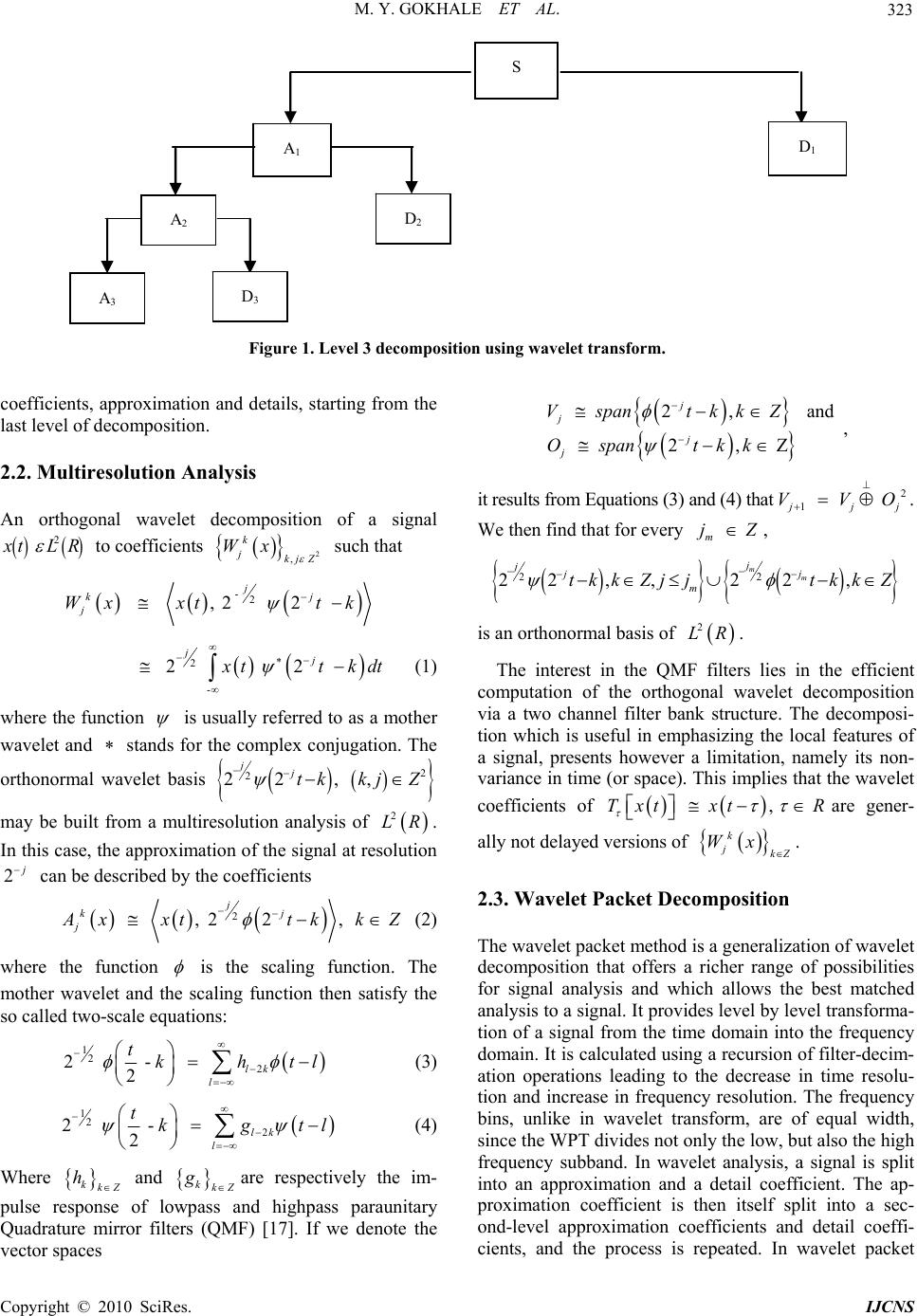 M. Y. GOKHALE ET AL. Copyright © 2010 SciRes. IJCNS 323 S D 1 A 1 A 2 D 2 A 3 D 3 Figure 1. Level 3 decomposition using wavelet transform. 2, and 2, Z j j j j Vspan tkkZ Ospan tkk , coefficients, approximation and details, starting from the last level of decomposition. 2.2. Multiresolution Analysis it results from Equations (3) and (4) that . We then find that for every , 2 1 jj VVO j m jZ An orthogonal wavelet decomposition of a signal 2 x tLR to coefficients 2 , k jkj Z Wx such that - 2 , 2 2 j kj j Wx xttk 2 22, , jj m tkkZj j 2 22, m m jjtkk Z is an orthonormal basis of 2 LR . 2 - 2 2 jj x ttk dt (1) where the function is usually referred to as a mother wavelet and stands for the complex conjugation. The orthonormal wavelet basis 2 2 22, , jjtkkjZ may be built from a multiresolution analysis of 2 LR. In this case, the approximation of the signal at resolution can be described by the coefficients 2j The interest in the QMF filters lies in the efficient computation of the orthogonal wavelet decomposition via a two channel filter bank structure. The decomposi- tion which is useful in emphasizing the local features of a signal, presents however a limitation, namely its non- variance in time (or space). This implies that the wavelet coefficients of , Txt xtR k jkZ Wx are gener- ally not delayed versions of . 2 , 22, j kj j A xxt tkk Z (2) 2.3. Wavelet Packet Decomposition The wavelet packet method is a generalization of wavelet decomposition that offers a richer range of possibilities for signal analysis and which allows the best matched analysis to a signal. It provides level by level transforma- tion of a signal from the time domain into the frequency domain. It is calculated using a recursion of filter-decim- ation operations leading to the decrease in time resolu- tion and increase in frequency resolution. The frequency bins, unlike in wavelet transform, are of equal width, since the WPT divides not only the low, but also the high frequency subband. In wavelet analysis, a signal is split into an approximation and a detail coefficient. The ap- proximation coefficient is then itself split into a sec- ond-level approximation coefficients and detail coeffi- cients, and the process is repeated. In wavelet packet where the function is the scaling function. The mother wavelet and the scaling function then satisfy the so called two-scale equations: 12 2 2 - 2lk l tkht l (3) 12 2 2 - 2lk l tkgt l (4) Where and are respectively the im- pulse response of lowpass and highpass paraunitary Quadrature mirror filters (QMF) [17]. If we denote the vector spaces kkZ hkkZ g 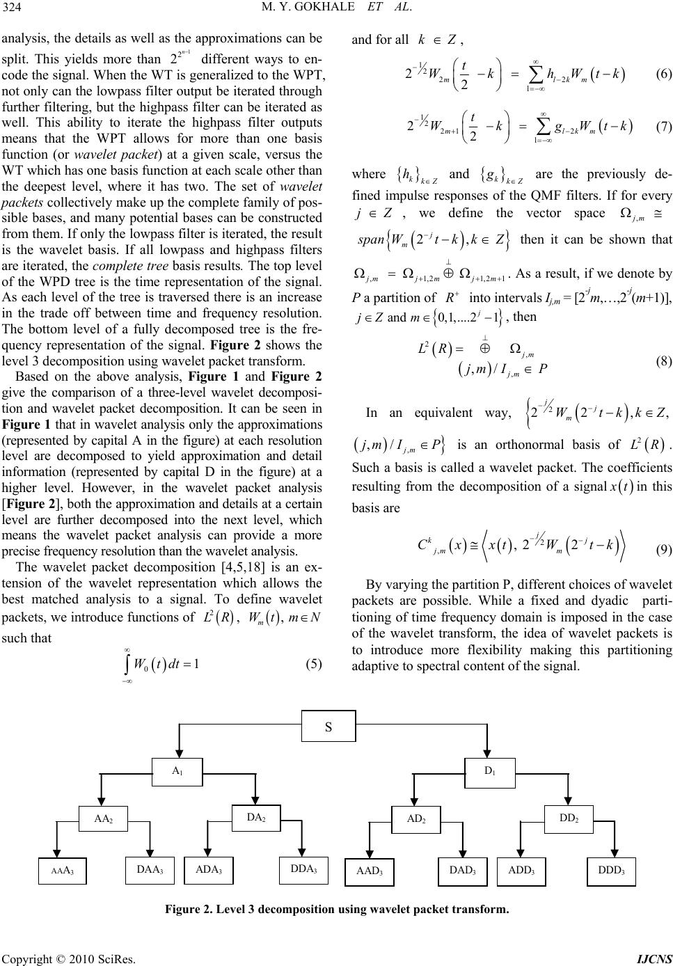 M. Y. GOKHALE ET AL. 324 analysis, the details as well as the approximations can be split. This yields more than different ways to en- code the signal. When the WT is generalized to the WPT, not only can the lowpass filter output be iterated through further filtering, but the highpass filter can be iterated as well. This ability to iterate the highpass filter outputs means that the WPT allows for more than one basis function (or wavelet packet) at a given scale, versus the WT which has one basis function at each scale other than the deepest level, where it has two. The set of wavelet packets collectively make up the complete family of pos- sible bases, and many potential bases can be constructed from them. If only the lowpass filter is iterated, the result is the wavelet basis. If all lowpass and highpass filters are iterated, the complete tree basis results. The top level of the WPD tree is the time representation of the signal. As each level of the tree is traversed there is an increase in the trade off between time and frequency resolution. The bottom level of a fully decomposed tree is the fre- quency representation of the signal. Figure 2 shows the level 3 decomposition using wavelet packet transform. 1 2 2n Based on the above analysis, Figure 1 and Figure 2 give the comparison of a three-level wavelet decomposi- tion and wavelet packet decomposition. It can be seen in Figure 1 that in wavelet analysis only the approximations (represented by capital A in the figure) at each resolution level are decomposed to yield approximation and detail information (represented by capital D in the figure) at a higher level. However, in the wavelet packet analysis [Figure 2], both the approximation and details at a certain level are further decomposed into the next level, which means the wavelet packet analysis can provide a more precise frequency resolution than the wavelet analysis. The wavelet packet decomposition [4,5,18] is an ex- tension of the wavelet representation which allows the best matched analysis to a signal. To define wavelet packets, we introduce functions of , 2 LR , m Wt mN such that 01Wtdt (5) and for all kZ , 12 22 l 2 2 mlk t Wk hWt m k (6) 12 21 2 l 2 2 mlk t WkgWt m k (7) where kkZ h and kkZ g are the previously de- fined impulse responses of the QMF filters. If for every jZ , we define the vector space , jm 2, j m s pan jm W t ,1 jm k ,2 k Z 1,21jm then it can be shown that R . As a result, if we denote by P a partition of into intervals Ij,m = [2-jm,…,2-j(m+1)], and 0,1,....21 j jZ m , then 2 , , ,/ jm jm LR jm IP (8) In an equivalent way, 2 22, jj m WtkkZ , , ,/ jm jm IP is an orthonormal basis of 2 LR. Such a basis is called a wavelet packet. The coefficients resulting from the decomposition of a signal x tin this basis are 2 ,, 22 j kj jm m CxxtW tk (9) By varying the partition P, different choices of wavelet packets are possible. While a fixed and dyadic parti- tioning of time frequency domain is imposed in the case of the wavelet transform, the idea of wavelet packets is to introduce more flexibility making this partitioning adaptive to spectral content of the signal. S D 1 AD 2 DD 2 AAD 3 DAD 3 ADD 3 DDD 3 A 1 AA 2 DA 2 AA A 3 DAA 3 ADA 3 DDA 3 Figure 2. Level 3 decomposition using wavelet packet transform. Copyright © 2010 SciRes. IJCNS  M. Y. GOKHALE ET AL. 325 In wavelet packet analysis, an entropy-based criterion is used to select the most suitable decomposition of a given signal. This means we look at each node of de- composition tree and quantify the information to be gained by performing each split [19]. The wavelets have several families. The most important wavelets families are Haar, Daubechies, Symlets, Coiflets, and biorthogo- nal. 3. Proposed Work The block diagram shown in Figure 3 gives the actual implementation of the method proposed in this paper. 1) Input tim e domain signal The system described above was simulated on a com- puter with floating point numbering system. The input time domain wave is pre-emphasized, low pass filtered with sampling frequency 8 K to 44.1 KHz range and 1– 10 sec duration samples. The time domain is digitized to 16 bits. Preprocessing: In this block unwanted noise is removed when the signal gets recorded with the help of various digital filter such as Low pass filter (LPF) with 3.4 KHz, Notch filter to remove the line frequency effect i.e. 50 Hz. Wavelet tr ansforms : In this block we applied the wavelet filter coefficients as low and high band and filter the input signal to en- hance the band energies. Decimation: As deals with the multi-rate analysis system the deci- mation factor helps to enhance the band level informa- tion from wavelet transform. We consider decimation by 2, 4 etc for our experiments. Analysi s Subband Feature Vectors: From the filtering results obtained with the 2 band system, we have extracted the various features from low pass and high pass band and then re-arranged with the desired format for further analysis part. Interpolation: Interpolation deals with up sampling the inverse wave- let filtering to reconstruct the original input signal. Inverse Wavelet transforms: Analysis of interpolated features is reordered with re- spect to the 2 bands system to extract the original con- tents from the feature vector for input signal synthesis purpose. Noise Removal: Input noisy signal is filtered with band stop filter with desired cut off frequency. Filtered output is further ap- plied to post processing. Post Processing: Final tuning is done in the post processing block. 2) Testing Setup Matlab programs were written to implement the struc- ture shown in Figure 3. Time domain signals in a *.wav format sampled at 8 KHz were used for all simulations. Results for different setups are given in the next section. Several examples of time domain signals of different sampling frequencies, with five wavelet filter families are given below. 3) Performance Evaluation Performance evaluation tests can be done by subjec- tive quality measures and objective quality measures. Objective measures provide a measure that can be easily implemented and reliably reproduced. Objective meas- ures are based on mathematical comparison of the origi- nal and processed time domain signals. The majority of objective quality measures quantify time domain quality of the signal in terms of a numerical distance measure. The signal to noise ratio is the most widely used method to measure time domain signal quality. It is calculated as the ratio of the signal to noise power in decibels. 2 10 2 10 logˆ n n sn SNR sn sn (10) where s(n) is the clean time domain signal and ŝ(n) is the processed time domain signal. Analysis subband Wavelet Packet Decimation Preprocessing Interpolation Inverse Wavelet Packet Transform Filter for noise removal Post processing Time domain Signal + Noise An alys is O/P Synthesis Figure 3. Block diagram of time domain signal using wavelet packet transform. C opyright © 2010 SciRes. IJCNS  M. Y. GOKHALE ET AL. 326 4. Results We have tested the 10 input samples with sampling fre- quency of 8 K on various wavelet filtering bank i.e. Haar, Db4, Symlet, dmey, etc. as shown in Tables 1, 3, 4, 7. We observe that SNR for wavelet packet analysis and synthesis after filtering is around 120 dB to 320 dB for level 1 decomposition, level 2 decomposition 120 dB to 310 dB, level 3 decomposition 115 dB to 310 dB and level 4 decomposition 115 dB to 305 dB. From Tables 2, 4, 6, 8 as per timing consideration the total time for analysis and synthesis is tabulated. We observe that total time for analysis and synthesis using wavelet filtering is around 8 sec to 25 sec. Table 1. SNR calculation for various mother wavelet level 1 decomposition. Sample Haar Db4 Sym5 dmey Coif5 T1 315.64 244.16 247.86 122.32 165.94 T2 315.58 244.16 247.86 122.28 165.95 T3 315.53 244.16 247.86 122.35 165.94 T4 315.55 244.16 247.86 122.34 165.94 T5 315.55 244.16 247.86 122.34 165.94 T6 315.53 244.16 247.86 122.35 165.94 T7 315.53 244.16 247.86 122.30 165.95 T8 315.53 244.16 247.86 122.35 165.94 T9 315.55 244.17 247.87 122.25 165.95 T10 315.54 244.16 247.86 122.32 165.95 Figure 4. Graphical presentation of SNR for various mo- ther wavelets. Table 2. Total time calculation (in seconds) for analysis and synthesis using wavelet filtering for level 1. Sample Haar Db4 Sym5 dmey Coif5 T1 8.10 8.31 9.15 9.40 8.96 T2 8.90 10.56 9.17 11.01 9.28 T3 8.53 9.43 9.32 13.45 10.40 T4 8.85 9.34 9.06 12.31 10.20 T5 8.39 9.01 8.59 11.90 9.29 T6 10.73 11.37 12.45 13.10 11.90 T7 11.48 12.03 13.07 13.28 13.18 T8 8.65 9.23 10.46 12.57 9.62 T9 9.59 10.65 10.20 11.40 11.26 T10 9.32 9.64 9.67 13.29 10.11 Table 3. SNR calculation of various mother wavelets for level 2 decomposition. SampleHaar Db4 Sym5 dmey Coif5 T1 310.41 232.64 247.31 121.37 165.81 T2 310.41 232.64 247.31 121.34 165.82 T3 310.40 232.64 247.31 121.36 165.81 T4 310.41 232.64 247.31 121.39 165.81 T5 310.38 232.64 247.31 121.36 165.81 T6 310.40 232.64 247.31 121.42 165.81 T7 310.40 232.64 247.31 121.33 165.82 T8 310.39 232.64 247.31 121.42 165.81 T9 310.40 232.65 247.31 121.25 165.82 T10 310.41 232.64 247.31 121.34 165.82 Figure 5. Graphical presentation of SNR for various mo- ther wavelets. Table 4. Total time calculation (in seconds) for analysis and synthesis using wavelet filte r ing for level 2. SampleHaar Db4 Sym5 dmey Coif5 T1 8.29 8.73 10.11 12.85 9.20 T2 10.10 11.06 11.57 14.64 11.21 T3 9.60 9.56 10.06 12.51 10.43 T4 8.93 10.43 9.48 13.95 11.67 T5 8.42 10.18 8.89 11.92 10.85 T6 11.82 13.51 12.48 15.62 13.00 T7 10.70 12.64 13.11 16.84 13.40 T8 9.45 10.53 9.82 13.28 10.56 T9 9.21 10.09 9.81 12.18 11.04 T10 10.75 10.98 11.09 14.25 10.71 Table 5. SNR calculation of various mother wavelets for level 3 decomposition. SampleHaar Db4 Sym5 dmey Coif5 T1 307.15 230.59 241.56 115.85 159.86 T2 307.15 230.60 241.56 115.84 159.86 T3 307.13 230.59 241.56 115.84 159.86 T4 307.12 230.59 241.56 115.86 159.86 T5 307.14 230.59 241.56 115.85 159.86 T6 307.14 230.59 241.56 115.88 159.86 T7 307.16 230.60 241.56 115.83 159.87 T8 307.15 230.59 241.56 115.87 159.87 T9 307.15 230.60 241.57 115.77 159.87 T10 307.14 230.60 241.56 115.83 159.86 Copyright © 2010 SciRes. IJCNS  M. Y. GOKHALE ET AL. 327 Figure 6. Graphical presentation of SNR for various Mot- her wavelets. Table 6. Total time calculation (in seconds) for analysis and synthesis using wavelet filtering for level 3. Sample Haar Db4 Sym5 dmey Coif5 T1 9.45 9.42 9.76 12.46 9.40 T2 10.35 11.70 10.57 15.64 11.01 T3 10.17 11.53 13.28 14.98 12.07 T4 10.11 11.48 12.21 16.54 12.40 T5 10.00 10.89 10.04 12.89 11.57 T6 11.84 13.73 13.21 18.04 14.68 T7 12.65 12.12 12.76 20.37 13.60 T8 10.53 11.20 10.87 15.43 11.86 T9 9.56 10.00 11.59 14.32 11.96 T10 10.32 10.48 11.96 16.68 13.42 Table 7. SNR calculation of various mother wavelets for level 4 decomposition. Sample Haar Db4 Sym5 dmey Coif5 T1 304.74 226.62 241.29 115.31 159.79 T2 304.74 226.62 241.29 115.29 159.79 T3 304.74 226.62 241.29 115.33 159.79 T4 304.73 226.62 241.29 115.37 159.79 T5 304.73 226.62 241.29 115.32 159.79 T6 304.73 226.62 241.29 115.37 159.79 T7 304.74 226.62 241.29 115.27 159.80 T8 304.75 226.62 241.29 115.36 159.79 T9 304.74 226.62 241.29 115.21 159.80 T10 304.74 226.62 241.29 115.30 159.80 Figure 7. Graphical presentation of SNR for various Mot- her wavelets. Table 8. Total time calculation (in seconds) for analysis and synthesis using wavelet filtering for level 4. SampleHaar Db4 Sym5 dmey Coif5 T1 9.95 10.90 10.76 14.92 12.26 T2 12.01 12.59 13.48 19.46 14.84 T3 12.12 12.81 14.79 22.09 12.53 T4 11.03 12.79 11.98 20.34 14.73 T5 11.34 12.37 12.54 16.79 13.09 T6 13.25 15.59 16.37 25.25 19.20 T7 14.51 15.40 17.39 25.89 17.98 T8 11.90 13.14 11.96 19.57 13.15 T9 12.09 13.17 12.51 20.01 15.48 T10 13.09 13.28 14.57 21.75 15.35 From Table 9, entropy which is a common measure of the efficiency of a signal transform is calculated using wavelet packet analysis is matched before decomposition and reconstruction. In Table 10, Band stop filtered signal is tabulated which removes the line frequency noise from the signal, it shows a reasonable SNR of 40–46 dB. Figure 8 shows the tree diagram associated with a depth-3 WPT. It reflects the structure of its correspond- ing hierarchical filter bank, such as the structure shown in Figure 2. Moving from top to bottom in the diagram Table 9. Entropy for 4 levels. SampleHaar/Db4/Sym5/dmey/Coif5 T1 21937 T2 32511 T3 29809 T4 34655 T5 29145 T6 49058 T7 51218 T8 32971 T9 34857 T10 37040 Table 10. SNR after removing noise. SampleHaar/Db4/Sym5/dmey/Coif5 T1 44.16 T2 44.41 T3 41.29 T4 44.52 T5 44.47 T6 44.85 T7 44.58 T8 40.39 T9 46.36 T10 41.89 C opyright © 2010 SciRes. IJCNS  M. Y. GOKHALE ET AL. 328 of Figure 8, frequency is divided into ever smaller seg- ments. Each line that emanates down and to the left of a node represents a lowpass filtering operation (h0), and each line emanating down and to the right a highpass filtering operation (h1). The nodes that have no further nodes emanating down from them are referred to as ter- minal nodes, leaves, or subbands. We refer to the other nodes as non-terminal, or internal nodes. As such, the tree node labeling scheme provides a simple mechanism for indicating the nodes in the tree that we can work with when imparting modifications on the signal. For the node (j,k), j denotes the depth within the transform (tree) and k the position. For example, at node (0,0) no filtering has taken place, and we simply have the original sequence of time samples. Lowpass filtering this will produce node (1,0) and highpass filtering with pro- duces (1,1). These filtering operations are equivalent to finding the correlation of the signal with the scaling function for node (1,0) and the correlation of the signal with the wavelet function for node (1,1). Going down the tree to the next depth, we see that (2,0) and (2,1) emanate from (1,0). From the filter perspective, the samples at (1,0) are applied to the filters and. Multiresolution is ach- ieved because the coefficients at (1,0) have been down sampled by two to achieve critical sampling. From the wavelet and scaling function perspective, the correlations between both and the samples of (1,0) are determined through this operation. Figure 9 shows how the block diagram wise analysis and synthesis is carried out. Figure 8. Wavelet packet tree for level 3 of decomposition. (a) (b) (c) (d) (e) (f) Figure 9. Input sample: (a) t7.w av; (b) For Haar wave let; (c) For Db4 wavelet; (d) For Sym5 wavelet; (e) For dmey wave- let; (f) line freq filter. Copyright © 2010 SciRes. IJCNS Please add units to Figure 9(a)-(f) -time (sec) or (min) or (hour)?  M. Y. GOKHALE ET AL. Copyright © 2010 SciRes. IJCNS 329 5. Conclusions We have presented a method for analysis and synthesis of time signals using wavelet packet filtering techniques. From this study we could understand and experience the effectiveness of wavelet packet transform in time signal analysis and synthesis. The performance of wavelet packet is appreciable while comparing with the discrete wavelet transform decomposition technique since wave- let packet analysis can provide a more precise frequency resolution than the wavelet analysis. It also has compact support in time as well as in frequency domain and adapts its support locally to the signal which is important in time varying signal. With wavelet packets we have a greater variety of options for decomposing the signal. The method presented is used for time as well as frequency analysis of time varying signals. From the results we conclude that the wavelet filtering find applications in the time domain analysis and synthesis era. In terms of signal quality, Haar wavelet has been seen to be the best mother wavelet. This is taken from the analysis of the signal to noise ratio (SNR) value around which is quite satisfactory for time varying signals. The system has been tested with various sampling frequencies for time domain samples which gave satisfactory output. Taking into consideration the signal quality and the time for analysis and synthesis it can be concluded that Haar wavelet is the best mother wavelet. Hence we conclude that the system will behave stable with wavelet packet filter and can be used for time signal analysis and syn- thesis purpose. 6. References [1] S. Mallat, “A wavelet tour of signal processing,” Second Edition, Academic Press, 1998. [2] D. Donoho, “De-noising by soft-thresholding,” IEEE Transactions on Information Theory, Vol. 41, pp. 613– 627, May 1995. [3] I. Daubechies, “Ten lectures on wavelets,” SIAM, New York, 1992. [4] J. W. Seok and K. S. Bae, “Speech enhancement with reduction of noise components in the wavelet domain,” IEEE International Conference on Acoustics, Speech and Signal Processing, Vol. 2, pp. 1323–1326, 1997. [5] P. V. Tuan and G. Kubin, “DWT-Based classification of acoustic-phonetic classes and phonetic units,” Interna- tional Conference on Spoken Language Processing, 2004. [6] E. P. A. Montuori, “Real time performance measures of low delay perceptual audio coding,” Journal of Electrical Engineering, Vol. 56, No. 3–4, pp. 100–105, 2005. [7] I. Daubechies, “Orthonormal bases of compactly sup- ported wavelets,” Communications on Pure and Applied Mathematics, Vol. 41, No. 7, pp. 909–996 , November 1998. [8] S. Mallat, “A theory for multiresolution signal decompo- sition: The wavelet representation,” IEEE Transactions on Pattern Analysis and Machine Intelligence, Vol. 11, No. 7, pp. 674–693, July 1989. [9] A. Grossman and J. Morlet, “Decompositions of Hardy functions into square integrable wavelets of constant shape,” SIAM Journals on Mathematical Analysis, Vol. 15, No. 4, pp. 723–736, July 1984. [10] R. Coifman and M. Wickerhauser, “Entropy-based algo- rithms for best basis selection,” IEEE Transactions on Information Theory, Vol. 38, No. 2, March 1992. [11] R. Learned, “Wavelet packet based transient signal clas- sification,” Master’s Thesis, Massachusetts Institute of Technology, 1992. [12] M. Wickerhauser, “Lectures on wavelet packet algo- rithms,” Technical Report, Department of Mathematics, Washington University, 1992. [13] R. Priebe and G. Wilson, “Applications of ‘matched’ wavelets to identification of metallic transients,” Pro- ceedings of the IEEE–SP International Symposium, Vic- toria, British Columbia, Canada, October 1992. [14] E. Serrano and M. Fabio, “The use of the discrete wavelet transform for acoustic emission signal processing,” Pro- ceedings of the IEEE–SP International Symposium, Vic- toria, British Columbia, Canada, October 1992. [15] T. Brotherton, T. Pollard, R. Barton, A. Krieger, and L. Marple, “Applications of time frequency and time scale analysis to underwater acoustic transients,” Proceedings of the IEEE–SP International Symposium, Victoria, Brit- ish Columbia, Canada, October 1992. [16] K. P. Soman and K. I. Ramachandran, “Insight into wavelets: From theory to practice,” 2nd Edition, PHI, 2005. [17] P. P. Vaidyanathan, “Multirate systems and filter banks,” Prentice Hall, New Jersey, 1992. [18] M. V. Wickerhauser, “INRIA lectures on wavelet packet algorithms,” Lecture Notes, pp. 31–99, June 1991. [19] MATLAB7.0. http://www.mathworks.com. |