Paper Menu >>
Journal Menu >>
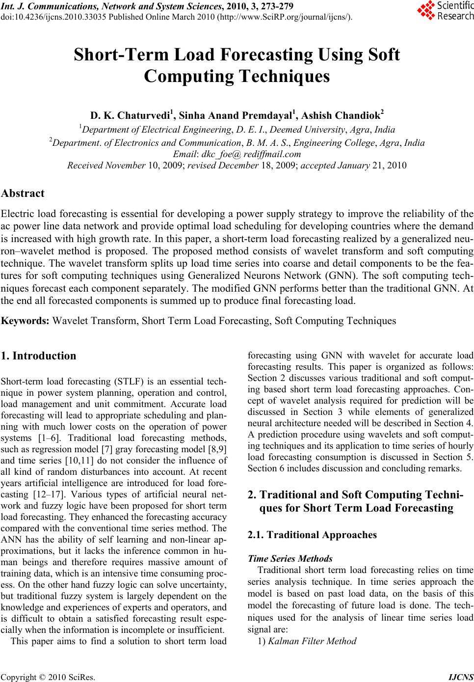 Int. J. Communications, Network and System Sciences, 2010, 3, 273-279 doi:10.4236/ijcns.2010.33035 blished Online March 2010 (http://www.SciRP.org/journal/ijcns/). Copyright © 2010 SciRes. IJCNS Pu Short-Term Load Forecasting Using Soft Computing Techniques D. K. Chaturvedi1, Sinha Anand Premdayal1, Ashish Chandiok2 1Department of Electrical Engineering, D. E. I., Deemed University, Agra, India 2Department. of Electronics and Communication, B. M. A. S., Engineering College, Agra, India Email: dkc_foe@ rediffmail.com Received November 10, 2009; revised December 18, 2009; accepted January 21, 2010 Abstract Electric load forecasting is essential for developing a power supply strategy to improve the reliability of the ac power line data network and provide optimal load scheduling for developing countries where the demand is increased with high growth rate. In this paper, a short-term load forecasting realized by a generalized neu- ron–wavelet method is proposed. The proposed method consists of wavelet transform and soft computing technique. The wavelet transform splits up load time series into coarse and detail components to be the fea- tures for soft computing techniques using Generalized Neurons Network (GNN). The soft computing tech- niques forecast each component separately. The modified GNN performs better than the traditional GNN. At the end all forecasted components is summed up to produce final forecasting load. Keywords: Wavelet Transform, Short Term Load Forecasting, Soft Computing Techniques 1. Introduction Short-term load forecasting (STLF) is an essential tech- nique in power system planning, operation and control, load management and unit commitment. Accurate load forecasting will lead to appropriate scheduling and plan- ning with much lower costs on the operation of power systems [1–6]. Traditional load forecasting methods, such as regression model [7] gray forecasting model [8,9] and time series [10,11] do not consider the influence of all kind of random disturbances into account. At recent years artificial intelligence are introduced for load fore- casting [12–17]. Various types of artificial neural net- work and fuzzy logic have been proposed for short term load forecasting. They enhanced the forecasting accuracy compared with the conventional time series method. The ANN has the ability of self learning and non-linear ap- proximations, but it lacks the inference common in hu- man beings and therefore requires massive amount of training data, which is an intensive time consuming proc- ess. On the other hand fuzzy logic can solve uncertainty, but traditional fuzzy system is largely dependent on the knowledge and experiences of experts and operators, and is difficult to obtain a satisfied forecasting result espe- cially when the information is incomplete or insufficient. This paper aims to find a solution to short term load forecasting using GNN with wavelet for accurate load forecasting results. This paper is organized as follows: Section 2 discusses various traditional and soft comput- ing based short term load forecasting approaches. Con- cept of wavelet analysis required for prediction will be discussed in Section 3 while elements of generalized neural architecture needed will be described in Section 4. A prediction procedure using wavelets and soft comput- ing techniques and its application to time series of hourly load forecasting consumption is discussed in Section 5. Section 6 includes discussion and concluding remarks. 2. Traditional and Soft Computing Techni- ques for Short Term Load Forecasting 2.1. Traditional Approaches Time Series Methods Traditional short term load forecasting relies on time series analysis technique. In time series approach the model is based on past load data, on the basis of this model the forecasting of future load is done. The tech- niques used for the analysis of linear time series load signal are: 1) Kalman Filter Method  D. K. CHATURVEDI ET AL. 274 The kalman filter is considered as the optimal solution to many data prediction and trend matching. The filter is constructed as a mean square minimization which re- quires the estimation of the covariance matrix. The role of the filter is to extract the features from the signal and ignore the rest part. As load data are highly non linear and non stationary, it is difficult to estimate the covari- ance matrix accurately [18]. 2) Box Jenkins Method This model is called as autoregressive integrated mov- ing average model. The Box Jenkins model can be used to represent the process as stationary or non stationary. A stationary process is one whose statistical properties are same over time, which means that they fluctuate over fixed mean value. On other hand non stationary time series have changes in levels, trends or seasonal behavior. In Box Jenkins model the current observation is weigh- ted average of the previous observation plus an error term. The portion of the model involving observation is known as autoregressive part of the model and error term is known as moving average term. A major obstacle here is its slow performance [19]. 3) Regression Model The regression method is widely used statistical tech- nique for load forecasting. This model forms a relation- ship between load consumptions done in past hour as a linear combination to estimate the current load. A large data is required to obtain correct results, but it requires large computation time. 4) Spectral Expansion Technique This method is based on Fourier series. The load data is considered as a periodic signal. Periodic signal can be represented as harmonic summation of sinusoids. In the same way electrical load signal is represented as summa- tion of sinusoids with different frequency. The drawback of this method is that electrical load is not perfect peri- odic. It is a non stationary and non linear signal with abrupt variations caused due to weather changes. This phenomenon results in the variation of high frequency component which may not be represented as periodic spectrum. This method is not suitable and also requires complex equation and large computation time. 2.2. Soft Computing Approach Soft computing is based on approximate models working on approximate reasoning and functional approximation. The basic objective of this method is to exploit the tol- erance for imprecision, uncertainty and partial truth to achieve tractability, robustness, low solution cost and best results for real time problems. 1) Artificial Neural Networks (ANN) An artificial neural network is an efficient information processing system to perform non-linear modeling and adaptation. It is based on training the system with past and current load data as input and output respectively. The ANN learns from experience and generalizes from previous examples to new ones. It is able to forecast more efficiently the load as the load pattern are non lin- ear and ANN is capable to catch trends more accurately than conventional methods. 2) Rule Based Expert Systems An expert system is a logical program implemented on computer, to act as a knowledge expert. This means that program has an ability to reason, explain and have its knowledge base improved as more information becomes available to it. The load-forecast model can be built us- ing the knowledge about the load forecast domain from an expert in the field. The knowledge engineer extracts this knowledge from the load domain. This knowledge is represented as facts and rules using the first predicate logic to represent the facts and IF-THEN production rules. Some of the rules do not change over time, some changes very slowly; while others change continuously and hence are to be updated from time to time [20]. 3) Fuzzy Systems Fuzzy sets are good in specialization, fuzzy sets are able to represent and manipulate electrical load pattern which possesses non-statistical uncertainty. Fuzzy sets are a generalization of conventional set theory that was introduced as a new way to represent vagueness in the data with the help of linguistic variable. It introduces vagueness (with the aim of reducing complexity) by eliminating the sharp boundary between the members of the class from nonmembers [21,22]. These approaches are based on specific problems and may represent randomness in convergence or even can diverge. The above mentioned approaches use either reg- ression, frequency component or mean component or the peak component to predict the load. The prediction of the load depends upon both time and frequency component which varies dynamically. In this paper, an attempt is made to predict electrical load that combines the above mentioned features using generalized neurons and wave- let. 3. Elements of Wavelet Analysis Wavelet analysis is a refinement of Fourier analysis [9– 15,23–29] which has been used for prediction of time series of oil, meteorological pollution, wind speed, rain- fall etc. [28,29]. In this section some important vaults relevant to our work have been described. The underly- ing mathematical structure for wavelet bases of a func- tion space is a multi-scale decomposition of a signal, known as multi-resolution or multi-scale analysis. It is called the heart of wavelet analysis. Let L2(R) be the space of all signals with finite energy. A family {Vj} of subspaces of L2(R) is called a multi resolution analysis of this space if Copyright © 2010 SciRes. IJCNS  D. K. CHATURVEDI ET AL. 275 1) intersection of all Vj, j = 1, 2, 3, ...... be non-empty, that is j jV 2)This family is dense in L2(R), that is, = L2(R) 3) f (x) V j if and only if f (2x) V j + 1 4) V1V2 ..... Vj V j + 1 There is a function preferably with compact support of such that translates (x – k) k Z, span a space V0. A finer space Vj is spanned by the integer translates of the scaled functions for the space Vj and we have scaling equation ()(2 1) k xa x (1) with appropriate coefficient ak, kZ. is called a scal- ing function or father wavelet. The mother wavelet is obtained by building linear combinations of . Fur- ther more and should be orthogonal, that is, ()() 0k,l,l,kZ (2) These two conditions given by (1) and (2) leads to conditions on coefficients bk which characterize a mother wavelet as a linear combination of the scaled and dilated father wavelets: ()= (2) k kz x bxk (3) Haar, Daubechies and Coefmann are some well known wavelets. Haar wavelet (Haar mother wavalet) denoted by ψ is given by 1,01 2 ()= 1,12<1 0,<0, >1 x x xx x (4) Can be obtained from the father wavelet 1, 01 ()= 0,0, 1 x xxx (5) In this case coefficients ak in (1) are a0 = a1 = 1 and ak = 0 for k 0, 1. The Haar wavelets is defined as a linear combination of scaled father wavelets (x) = (2x) – (2x – 1) which means that coefficients bk in (3) are b0 = 1, b1 = –1 and bk = 0 otherwise, Haar wavelets can be interpreted as Daubechie’s wavelet of order 1 with two coefficients. In general Daubechies’ wavelets of order N are not given analytically but described by 2N coeffi- cients. The higher N, the smoother the corresponding Daubechies’ wavelets are (the smoothness is around 0-2N for greater N). Daubechies’ wavelets are constructed in a way such that they give rise to orthogonal wavelet bases. It may be verified that orthogonality of translates of and , requires that k k a = 2 and = 2. kk b It is quite clear that in the higher case the scaled, trans- lated and normalized versions of are denoted by /2 , 22 jj jk tx k (6) With orthogonal wavelet the set { j, k | j, k Z} is an orthogonal wavelet basis. A function f can be rep- resented as j,k j,kj,k jZkZ f =c (, c< f >) (7) The Discrete Wavelet Transform (DWT) corresponds to the mapping f cj,k. DWT provides a mechanism to represent a data or time series f in terms of coefficients that are associated with particular scales [24,26,27] and therefore is regarded as a family of effective instrument for signal analysis. The decomposition of a given signal f into different scales of resolution is obtained by the ap- plication of the DWT to f. In real application, we only use a small number of levels j in our decomposition (for instance j = 4 corresponds to a fairly good level wavelet decomposition of f). The first step of DWT corresponds to the mapping f to its wavelet coefficients and from these coefficients two components are received namely a smooth version, nam- ed approximation and a second component that corre- sponds to the deviations or the so-called details of the signal. A decomposition of f into a low frequency part a, and a high frequency part d, is represented by f = a1 + d1. The same procedure is performed on a1 in order to obtain decomposition in finer scales: a1 = a2 + d2. A recursive decomposition for the low frequency parts follows the directions that are illustrated in Figure 1. The resulting low frequency parts a1, a2, ..... an are ap- proximations of f, and the high frequency parts d1, d2, ..... dn contain the details of f. This diagram illustrates a wavelet decomposition into N levels and corresponds to 123 1 N NN f ddddda (8) In practical applications, such decomposition is ob- tained by using a specific wavelet. Several families of wavelets have proven to be especially useful in various applications. They differ with respect to orthogonality, smoothness and other related properties such as vanish- ing moments or size of the support. Figure 1. Wavelet decomposition in form of coarse and de- tail coeffici e nts. C opyright © 2010 SciRes. IJCNS  D. K. CHATURVEDI ET AL. 276 4. Neuro Theory of Generalized Neuron Model The following steps are involved in the training of a summation type generalized neuron as shown in Figure 2. 4.1. Forward Calculations Step 1: The output of thepart of the summation type generalized neuron is 1 *_ 1 1 s snet Oe (9) where _iio s netW XX Step 2: The output of the part of the summation type generalized neuron is 2 *_ ppi net Oe (10) where _* ii o pinetW XX Step 3: The output of the summation type generalized neuron can be written as *(1 )* pk OO WOW (11) 4.2. Reverse Calculation Step 4: After calculating the output of the summation s_bias Input, Xi pi_bias Outpu t, Op k s _ bias Output, O pk Input, Xi pi_bias Figure 2. Learning algorithm of a summation type general- ized neuron. neural network, it is compared with the Then, the uared error for patterns is type generalized neuron in the forward pass, as in the feed-forward desired output to find the error. Using back-propagation algorithm the summation type GN is trained to minimize the error. In this step, the output of the single flexible summation type generalized neuron is compared with the desired output to get error for the ith set of inputs: Error () iii EYO (12) sum-sq convergence of all the 2 05 p i E.E (13) A multiplication factor of plify the calculations. ron 0.5 has been taken to sim- Step 5: Reverse pass for modifying the connection strength. 1) Weight associated with the1and 2 part of the summation type Generalized Neu is: ()( 1)Wk WkW (14) where () i k WOOX (1)Wk and () ii kYO ts associated withe inputs of th2) Weigh the 1part of the summation type Generalized Neuron are: ()( 1) ii i Wk WkW (15) where (1 ij i WXiWk) and (1)* jk WOO s associated with the input of the part of the summation type generalized Neuron are: 3) Weight ()( 1) ii i Wk WkW (16) (1 ij i WXiWk where ) O and (1) * (2*_) * jk Wpinet Mcomentum factor for better convergene. Ranged by expe d Neuron–Wavelet Approach en sed to predict the electrical load. In this approach, Dau- Learning rate. from 0 to 1 and is determine of these factors is rience. . Generalize5 The Generalized Neuron–Wavelet approach has be u bechies wavelets Db8 have been applied in the decom- position for the give data pattern. There are four wavelet coefficients are used. All these wavelet coefficients are time dependent (the first three wavelet coefficients from Copyright © 2010 SciRes. IJCNS  D. K. CHATURVEDI ET AL. 277 - re 1 d1 to d3 and the coarse approximation a3. These coeffi- cients are illustrated in the Figure 3. We observe the substantial difference of variability of the signals at dif- ferent levels. The higher is the wavelet level, the lower variation of the coefficients and easier prediction of them. Our main idea is to substrate the prediction task of the original time series of high variability by the prediction of its wavelet coefficients on different levels of lower variability’s, and then using Equation (4) for final pre- diction of the power load at any time instant n. Since most of the wavelet coefficients are of lower variability we expect the increase of the total prediction accuracy. The wavelet tool available in Matlab is used for the process of wavelet decomposition of the time series rep senting average of the power load data for 120 hours. This step involves several different families of wavelets and a detailed comparison of their performance. In our case, The Daubechies wavelets of order 8 are performed. Three level wavelet decomposition of the given time series XN = f : is performed 33 2 f addd (17) The smooth part of f is stored in a3 ferent levels are captured by d, d, de , and details on dif- d. Consequently a 1 2 3 composition of the time series in three different scales is obtained. Figure 4 illustrates the decomposition of the original signals. The forecasting procedure methodology explained in Section 4 is used to predict the next value. The basic idea is to use the wavelet transforms and pre- dict the data by soft computing techniques for individual coefficients of wavelet transform represented by a3, d1, d2, d3. The input to the architecture to predict the wavelet coefficients is explained in Figure 5. Figure 4. Mechanism for forecasting Procedure. Figure 5. Actual and pr edicted training output using gener alized neuron model (GNN). load at an instant (i) is given y - The total predicted power b 1234 F ififififi (18) . Results and Discussions ollected for 120 hours om Gujarat system and normalized them in the range 6 The electric load data have been c fr 0–1. The Daubechies wavelet Db8 is used for decompo- sition and the wavelet coefficients d1–d3 and a3 have been calculated. The trend of coefficients has been used for GN training and predicting the wavelet coefficients for future loads. So wavelet is used to extract the feature coefficients from data and then GN is implemented to predict the trend of the wavelet coefficient. The results of GN and actual load have been compared and shown in Figure 3. Wavelet decomposition of hour load data into wavelet coeff ic ient. C opyright © 2010 SciRes. IJCNS  D. K. CHATURVEDI ET AL. 278 Figures 5 and 6. The root means square error for training and testing results are .1127 and .1152 mega watts (MW) as in Table 1. When using generalized neuron and wave- let conjunction model, training each coefficient and combining to get the predicted output, a very high im- provement is obtained in both training and testing results as shown in Figures 7 and 8. The root means square er- ror for training and testing data are .0554 and .0763 re- spectively as in Table 1. The improvement in the results shows that accuracy of forecasting increases in the com- bined model and can give correct output for short term load forecasting. Figure 6. Actual and predicted testing output using gee alized neuron model (GNN). GNN Wavelet chnique. pe Min. Error (Mw) Max. Error (Mw) RMSE (Mw) n r - Table 1. Comparison between GNN and te Ty GNN (training) 0.10009520.3663 0.1127 GNNW(training) 0.002184 0.1706 0.0554 GNN(testing) 0.1306 0.2094 0.1152 G NNW(testing) 0.00462 0.1913 0.0673 Figure 8. Actual and predicted testing output using gene alized neuron wavelet model (GNNW). s, J. B. Theocharis, S. J. Kiartzis, and A. G. Bakirtzis, “A novel approach to short-term load fore- recasting tric-load forecast using ANN and ARI- fuzzy neural asting technique,” IEEE Trans- rt the IEEE, Vol. 75, No. 1212, pp. ating electrical machines plications in science, analysis of gravity waves,” The Arabian Journal r- . References 7 1] S. E. Papadaki[ casting using fuzzy neuralnetworks,” IEEE Transactions on Power Systems, Vol. 13, pp. 480–492, 1998. [2] D. K. Chaturvedi, P. S. Satsangi, and P. K. Kalra, “Fuzz- ified neural network approach for load fo problems,” International Journal on Engineering Intelli- gent Systems, CRL Publishing, U. K., Vol. 9, No. 1, pp. 3–9, March 2001. [3] A. A. Eidesouky and M. M. Eikateb, “Hybrid adaptive techniques for elec MA,” IEE Proceedings–Generation, Transmission and Distribution, Vol. 147, pp. 213–217, 2000. [4] A. G. Bakirtzis, J. B. Theocharis, S. J. Kiartzis, and K. J. Satsios, “Short term load forecasting using networks,” IEEE Transactions on Power Systems, Vol. 10, pp. 1518–1524, 1995. [5] S. Rahman and O. Hazim, “A generalized knowledge- based short-term load forec actions on Power Systems, Vol. 8, pp. 508–514, 1993. [6] D. K. Chaturvedi, M. Mohan, R. K. Singh, and P. K. Kalra, “Improved generalized neuron model for sho term load forecasting,” International Journal on Soft Computing–A Fusion of Foundations, Methodologies and Applications, Springer–Verlag, Heidelberg, Vol. 8, No. 1, pp. 10–18, April 2004. [7] G. Gross and F. D. Galiana, “Short term load fore- casting,” Proceedings of 1558–1573, December 1987. [8] D. K. Chaturvedi, P. S. Satsangi, and P. K. Kalra, “New neuron models for simulating rot and load forecasting problems,” International Journal on Electric Power System Research, Elsevier Science, Ire- land, Vol. 52, pp. 123–131, 1999. [9] P. S. Addision, “The illustrated wavelet transform hand- book: Introductory theory and ap engineering medicine and finance,” IOP Publishing LTD, 2002. [10] Z. Can, Z. Aslan, and O. Oguz, “One dimensional wave- let real Figure 7. Actual and pr edicted training output using gener- alized neuron wavelet model (GNNW). Copyright © 2010 SciRes. IJCNS  D. K. CHATURVEDI ET AL. Copyright © 2010 SciRes. IJCNS 279 rm of meteorological parameters and gravity , San Diago, 1994. l world and systems,” teorological tick, Mass, 1995. power system analysis and contro nd control,” Holden-Day, San Frans ort-term load forecasting techniques,” IEEE Trans logic and neural network handbook,” certainty and ar and E. Foufoula–Georgiou, “Wavelet analysis f signal processing,” Acade- d A. H. Siddiqi, “Mathema- pplied functional analysis,” Maral Dek- in, W. Freeden, U. Mosco, and S. . Garanty, “Forecasting of the daily haos, “Wavelet eters, and Wellesley, “Adap- for Science and Engineering, Vol. 29, No. 2, pp. 33–42, 2004. [11] Z. Can, Z. Aslan, O. Oguz, and A. H. Siddiqi, “Wavelet transfo waves,” Annals Geophysics, Vol. 23, pp. 650–663, 2005. [12] I. Daubechies, “Ten lectures on wavelets,” SIAM, Phila- delphia, 1992. [13] A. F. Georgiou and P. Kumar, “Wavelet in geophysics,” Academic Press [14] K. M. Furati, M. Z. Nashed, and A. H. Siddiqi, “Mathe- matical models and methods for rea mic P Chapman and Hall/CRC, Taylor and Francis Group, Boca Raton, London, New York, Singapore, 2006. [15] Z. Z. Hu and T. Nitta, “Wavelet analysis of summer rain- fall over north China and India,” Journal Me tica Society of Japan, Vol. 74, No. 6, 1996. [16] J. S. R. Jang and N. Gulley, “Fuzzy logic toolbox,” The Mathworks Inc., 24 Prime Park Way, Na [17] J. S. R. Jang and C. T. Sun, “Neuro-fuzzy modeling and control,” Proceedings of the IEEE, Vol. 83, No. 3, pp. 378–406, 1995. [18] A. K. Mahalanabis, D. P. Kothari, and S. I. Ahson, “Computer aidedl,” me Tata McGraw Hill Publishing Company Limited, New Delhi, 1988. [19] G. E. Box and G. M. Jenkins, “Time series analysis: Forecasting aisco, -based prediction of oil prices,” Solution and Fractals, Vol. 25, pp. 265–275, 2005. [30] M. V. Wickerhauser, A. K. P 1976. [20] I. Moghram and S. Rahman “Analysis and evaluation of five sh- ted actions on Power Systems, Vol. 4, pp. 1484–1491, Oct- ober 1989. [21] C. H. Chen, “Fuzzy McGraw Hill Computer Engineering, 1996. [22] G. J. Klis and T. A. Folger, “Fuzzy sets un information,” Prentice Hall of India Private Limited, 1993. [23] P. Kum for geophysical applications,” Reviews of Geophysics, Vol. 33, pp. 385–412, 1997. [24] S. Mallat, “A wavelet tour o ress, NewYork, 1998. [25] P. Manchanda, J. Kumar, an l methods for modeling price fluctuations of financial time series,” Journal of Franklin Institute, Vol. 344, pp. 613–636, 2007. [26] A. H. Siddiqi, “A kar, New York, 2004. [27] A. H. Siddiqi, G. Kov Stephan, “Theme issue on wavelet fractal in science and engineering,” Arabian Journal for Science and Engi- neering, KFUPM. [28] O. Stanislaw and K teorological pollution using wavelet and support vector machine,” Engineering Application of Artificial Intelligence, Vol. 20, pp. 745–755, 2007. [29] S. Yousefi, I. Weinrich, and D. Reinarz–C analysis from theory to software,” 1994. |