J. Service Science & Management, 2010, 3 : 16 -22
doi:10.4236/jssm.2010.31002 Published Online March 2010 (http://www.SciRP.org/journal/jssm)
Heuristics for Production Allocation and Ordering
Policies in Multi-Plants with Capacity
Jie Zang1,2, Jiafu Tang1
1School of Information Science and Engineering, Northeastern University, Shenyang, China; 2School of Information, Liaoning
University, Shenyang, China.
Received October 19th, 2009; revised November 27th, 2009; accepted January 5th, 2010.
ABSTRACT
Joint decisions in production allocation and ordering policies for single and multiple products in a produc-
tion-distribution network system consisting of multiple plants are discussed, production capacity constraints of
multi-plants and unit production capacity for producing a product are considered. Based on the average total cost in
unit time, the decisive model is established. It tries to determine the production cycle length, delivery frequency in a
cycle from the warehouse to the retailer and the economic production allocation. The approach hinges on providing an
optimized solution to th e joint decision model through the heuristics methods. The heuristic algorithms are proposed to
solve the single-product joint decision model and the multi-products decision prob lem. Simulations on different sizes of
problems have shown that the heuristics is effective, and in general more effective than Quasi-Newton method (QNM).
Keywords: Joint Decisions, Production-Distribution; Multiple Plants, Capacitated, Heuristic Algorithm
1. Introduction
In the past, logistic decision among material procurement
management, production and distribution were made in
isolation. Previous studies have examined production,
transportation and inventory separately. These major ac-
tivities are closely related with each other and should be
coordinated effectively to enhance its profit in today’s
competitive market. Uncoordinated and isolated deci-
sion-making among functional related activities in supply
chain system may weaken its system-wide competitive-
ness. Hence, more efforts are now being made to inte-
grate coordinate production and distribution, production
and transportation, production and inventory, as well as
transportation and inventory in the form of supply chain
management.
King [1] described the implementation of a coordi-
nated production-distribution system, a major tire
manufacturer with four factories and nine major dis-
tribution centers. Williams [2] considered the problem
of joint scheduling of production and distribution in a
complex network, the objective of the problem was to
minimize average production and distribution cost per
period. Hill [3] discussed production-delivery policies
in a single manufacturer and a single retailer. David [4]
attempted to identify lot sizing and delivery schedul-
ing in a single manufacturer and a single retailer sys-
tem. Kim [5] discussed the production and ordering
policies in a supply chain consisting of a single manu-
facturer and a single retailer. He proposes an efficient
heuristic algorithm to determine the near optimal pro-
duction allocation ratios. Kim [6] extended their paper
and develops joint economic production allocation,
lot-sizing, and shipment policies in a supply chain
where a manufacturer produces multiple items in mul-
tiple production lines and ships the items to the re-
spective retailers. Their formulations are often based
on economic order quantity (EOQ) and mathe- matical
programming. Accordingly, the corresponding solu-
tion methods are EOQ [7,8], heuristics [5,6,9] and
decomposition [10,11].
In recent studies, model for coordinating production-
distribution network systems have tended to focus on
joint decisions on all activities. More complicated inte-
grated decisions on production, transportation, and in-
ventory have received relatively little attention, as in [12]
and [13]. Tang [12] discussed an integrated decision on
production assignment, lot-sizing, transportation, and
order quantity for a multiple-supplier/multiple-destin-
ations logistics network in a global manufacturing system
and proposed a heuristics to solve medium and large-
scale integrated decision problems. Yung [13] attempted

Heuristics for Production Allocation and Ordering policies in Multi-Plants with Capacity 17
to tackle joint decisions in assign ing production, lot-size,
transportation, and order quantity for sing and multiple
products in a production-distribution network system
with multiple suppliers and multiple destinations. He
provided an optimized so lution to so lve the jo int decision
model through a two-layer decomposition method that
combines several heuristics.
This paper addresses the issue of how to effectively
allocate production requirement to multiple plants in sup-
ply chain system. Kim [5,6] discussed the production and
ordering policies in a supply chain consisting of a single
manufacturer with multiple plan ts and a single retailer or
multiple retailers. The retailers place orders based on the
EOQ-like policy, and the multiple plants produce de-
mand requirement from the retailers. Each of multiple
plants has its production and tran sfer rates. In real life, all
the plants in the manufacturer have production capacity
constraints. All the plants should produce within its ca-
pacity to meet the demands of the retailers. The problem
discussed in this paper extends the model proposed by
[5,6], and production capacity constraints of multi-plants
and unit production capacity for producing a product are
considered in the model. The heuristics methods have
been developed to solve the problem with single product
and multiple products, respectively.
In this paper, the model for a single product will be dis-
cussed in Section 2, followed by detailed discussion to
solve multiple products in Section 3. One illustrated ex-
ample with several testing problems and their respective
simulation results and analyses are presented in Section 4.
2. Formulations and Heuristics with Single
Product
2.1 Problem Formulations
In a global manufacturing enterprise, there are plants
each producing multiple parts and multiple assemblies
that serve multiple assembly plants in a year, or alterna-
tively, each assembly plant demands multiple parts from
many different suppliers. Hence, such a global manufac-
turing enterprise can be formulated as a combined pro-
duction-distribution network consisting of multiple sup-
pliers and multiple destinations. In this paper, we con-
sider a production-distribution network composed of a
single manufacturer with multiple plants and multiple
retailers. The retailers are given annual demand of the
product. To meet the annual demands of the product, the
manufacturer procures the materials and multi-plants
produce within their capacity in the manufacturer. The
multi-plants of the manufacturer have their production
rate. Th e fin ished produ cts ar e tr ansf err ed to the co mmon
warehouse at the plants’ transfer rate. Finally, the ware-
house delivers the ordered lots of a fixed size to the re-
tailer periodically. The network is shown in Figure 1.
The cost components considered include two parts, the
first part is the ordering cost from raw materials, the pro-
Supplier
Procuremen
inventory
Plant1
Plant2
Plant
。。。
Warehouse
Retailer1
Retailer2
Retailer n
。。。
Figure 1. Production-distribution network
duction setup cost, the ordering cost at the warehouse, and
the ordering cost of the retailer; the second part is the
holding costs for raw materia ls, work-in-process invento-
ries, finished items at the warehouse and the retailer.
Assume that there are mplants in a manufacturer,
where each of the plants is indicated by the subscripts j.
The following notations and d ecision vari ables are applied.
j
P= annual production rate at plantj (unit/year)
j
Q= annual production capacity at plantj (year)
j
d= annual transfer rate from plantjto the warehouse
(unit)
j
u= production capacity needed to produce unit prod-
uct at plant j (year)
j
h= holding cost for work-in-pro cesses at plant j ($)
p
S= production setup cost at the manufacturer ($)
m
A
=ordering cost for raw materials at the manufac-
turer ($)
w
A
= order handling cost for finished products at the
warehouse ($)
r
A
= ordering cost at the retailer ($)
m
H
= holding cost for raw materials at the manufac-
turer ($)
w
H
= holding cost for finished products at the ware-
house ($)
r
H
= holding cost for finished products at the retailer ($)
D=demand rate in units at the retailer (unit/year)
T= decision variable, production cycle length at the
manufact ur er (year)
m= decision variable, delivery frequency in a produc-
tion cycle from the warehou se to the retailer
1
( ,...,)
j



decision variable, production allocation
for multiple plants
These notations will be extended in Section 3 to in-
clude multiple products. Accordingly, from the above
parameters and decision variables, j
jdD
 and
j
j
Pd should be satisfied for the relevance of the pro-

Heuristics for Production Allocation and Ordering policies in Multi-Plants with Capacity 18
posed model.
2.2 Joint Decision Model for a Single Product
The average cost components considered in this problem
include two parts, the first part is the ordering cost; the
second part is the holding costs these two parts of the
costs are denoted by F1 (T, m) and F2 (m,

) respectively.
In a production cycle has m delivery from the warehouse
to the retailer, so the ordering cost F1 (T, m) are given as
1(, )[()()]/ mp wr
F
TmA SmA AT  (1)
For the second part of the co sts, the average inventor y
levels for raw materials, work-in-process in plant (j),
and finished products at the warehouse and the retailer
over the production cycle are denoted by Im, Ij, Iw and Ir,
respectively. Im and Iw can be derived by the appendix of
Reference [5]. From the decision variables, we can de-
rived the production lot size is DT, and the apportioned
production lot size for plant i is jDT

. During a pro-
duction cycle, the production time is /
ii
DT P

, the deliv-
ery time is /
jj
DT d

, as illustrated in Figure 2. I t can be
shown that, the average inventory for work-in-process Ij is
22
11 1
[( /)( /)]
22
(/2)[(/)(1/)]
jjjjjjj
jj jj
I
DT dDTDTPDT
T
DTdd P




Hence, Im, Ij, Iw and Ir [5] a re gi ven a s
22
1
(/2) /
n
mjj
i
I
DT P 

 (2)
22
(/2)[(/)(1/)]
j
jj jj
I
DTdd P   (3)
22
1
(/2)(11/)( /2)/
n
wjj
i
I
DTmD Td 


(4)
/2
r
I
DT m (5)
Hence, the holding cost F2(m,

) are given as
21
(,) n
mmj jwwrr
j
F
mHI hIHIHI 

 
 (6)
Substituting (2)–(5) into (6), we can obtain
Figure 2. Inventroy trajectory for work-in-process in plant j
2
21
(,) (/2)[()/]
where H
n
wwr jj
j
jm wj
j
jj
FmDTHHHmDH
hHH h
Pd







(7)
The integrated decisions of the economic production
allocation and delivery policies are expressed as the fol-
lowing model:
Min W= F1(T, m) +F2(m,

)
2
1
[() ()]/
(/2)[ ()/]
mp wr
n
wwr jj
j
AS mAAT
DTHHHmDH


 


s.t. 1
j
j
 

(9)
0 /1,2,...,
jj
dD jn


 (10)
0 /1,2,...,
jj j
QDu jn


 (11)
In this model, (8) is the objective of minimizing the
average ordering and holding cost for raw materials,
work-in-process, finished products at the warehouse and
the retailer. The constraint (9) is the allocation vector for
multiple plants. The constraints (10) and (11) should be
satisfied by definition, respectively .
2.3 Heuristics Solution Procedures
The model is a fractional nonlinear programming model
that is neither convex nor concave and is difficult to be
solved. So we transform this model with the decision
variables (T, m ,

) into a more simplified and equivalent
problem with a decision variable

, the last transformed
problem is computed using a heuristic procedure.
First, the problem is strictly convex with respect to T,
thus the optimal cycle length T*(m,

) for a fixed pair of
m and

can be uniquely derived by solving dW/dT=0:
1/2
2
1
2[() ()]
T*
[()/()]
mp wr
n
wwr jj
j
AS mAA
HHHmDH D 





 







 



 (12)
Substituting T* into (8), we can derive E(m,

):
21/2
1
(,)(*,,)
{2[() ()]
[()/()]}
mp wr
n
wwr jj
j
EmWT m
AS mAA
HHHmDH D






 

(13)
For (13), we can derive:
2
1
(/)[() ()]
[()/( )]
mP wr
n
wwr jj
j
SmA SmA A
H
HHmDHD




 
 
(14)
(8)

Heuristics for Production Allocation and Ordering policies in Multi-Plants with Capacity 19
We can obtain (15) for fixed

:
n2
i1
2
2
23
(/) ()[ ]
()()
2( )()
(/)
wrw jj
mpw r
mpw r
dS mAAH DH
dm
ASHH
m
ASHH
dSm
dm m




 





(15)
Since )/(
2
 mSd /2
dm >0, we can obtain m from
dS/dm=0 and is given by
n21/2
1
() {()()/()
[()]}
mpw rwr
wjj
j
mASHHAA
HDH



 
 (16)
Since other terms in (17) are constant regardless of

except 2
1
n
j
j
jDH


, we reformulate the next problem
equivalently as follows:
2
1
()
s.t. (9),(10),(11)
n
j
j
j
MaxG H




This problem belongs to the class of quadratic maxi-
mization problems subject to linear constraints with a
positive definite quadratic term. Reference [14] has
proved it is an NP-hard problem. Since this problem aims
to assign production allocation
j

, a heuristic procedure
is proposed as follows to solve it.
The heuristic algorithm steps
Step1. Resequence Hi in the descending order, such
that 123 m
H
HH H;
Step2. Let t be the current index number of the plant to
be assigned, and 1
t
ti
i
R


be the total amount of the
production allocation t=0, Rt =0;
Step3. t=t+1 assignment to production to the tth plant
point:
If Rt-1<1 set
1
min{1,/ ,/}
ttttt
RdDQDu



1tt t
RR



Else 1 0,
tttt
RR




End if
Step4. If t<m , go to Step 3; else, go to Step5;
Step5. Calculate the MaxG(

), then stop.
After deriving

*, we can obtain m* and T* from (16)
and (12).
3. Joint Decisions for Multiple Products
3.1 Formulation with Multiple Products
In many real cases, the manufacture often produces multi-
ple products to meet the need of the retailers. In this pro-
duction-distribution network of multiple products, the
main issue is how joint decisions can be made annually on
production cycle length, delivery frequency and produc-
tion allocation at a minimal average cost to the network.
To derive the solution, the notations are defined as follows:
Pij = annual production rate for product i at plant j
(unit/year)
Qij = annual production capacity for product i at plant j
(year)
dij = annual transfer rate for product i from plant j to
the warehouse (unit)
uij = production capacity needed to produce unit prod-
uct i at plant j (year)
hij = holding cost for product i at plant j($)
Si = production setup cost for product i at the manu-
facturer ( $)
R
i
A
= ordering cost of raw materials for product i($)
W
i
A
= order handling cost for finished product i at the
warehouse ($)
C
i
A
= ordering cost for product i at the retailer ($)
R
i
H
= holding cost of raw materials for product i($)
W
i
H
= holding cost for finished product i at the ware-
house ($)
C
i
H
= holding cost for finis hed product i at the retailer ($)
Di = demand rate for product i (unit/year)
T = decision variable, production cycle length at the
manufacture r ( year)
mi = decision variable, delivery fr equency for product i
in a production cycle from the warehouse to the retailer
ij

= decision variable, production allocation for prod-
uct i in plant j
Similar to the average cost structure of a single prod-
uct, the ordering costs and the holding costs are repre-
sented as follows, respectively:
1(, )[()()]
RWC
i iiiii
i
F
TmASm AAT

(18)
The second part is the holding costs for raw materials,
work-in-process inventories, finished items at the ware-
house and the retailer. They are denoted by ,,
R
iij
I
I
,
i
WC
i
I
I respectively
22
1
(/2) /
n
R
ii ijij
j
I
DT P 

 (19)
22
(/2)[(/)(1/)]
ijiijijij ij
j
I
DTdd P  

(20)
22
1
(/2)(11/)( /2)/
i
n
Wiiiijij
j
I
DTmD Td 


(21)
/2
C
ii i
I
DT m (22)
Hence, the holding cost 2(,)
iij
Fm

are given as

Heuristics for Production Allocation and Ordering policies in Multi-Plants with Capacity 20
2(,) i
R
RWWCC
iijiiijij iii
iiji i
FmHIhI HIHI  
 
(23)
Substituting (19)–(22) into (23), we can obtain
2
2(,)(/2)[ ()/]
WWC
iiji iiiiiijij
ij
FmTDHHHm DH

 

(24)
()/()/
RW
ijijiijiij ij
H
hHP Hhd (25)
The integrated decisions of the economic production
allocation and delivery policies are expressed as the fol-
lowing model:
12
2
min(,)(,)
[() ()]
(/2) [ ()/]
iiij
RWC
ii ii i
i
WWC
iiiiiiij ij
ij
FFTmFm
ASmAAT
TDHHHmDH







(26)
.1
ij
j
s
ti  
 (27)
0/,
ijij i
dD ij

  (28)
0/
iji jiij
QDu j

  (29)
3.2 Heuristics Method for Multiple Products
The model is a fractional nonlinear programming model
that is the same as the model with the single product. It
can be solved by traditional nonlinear programming
techniques, such as GINO, gradient search methods,
where only the local optimal solution may be found. A
heuristics is proposed to solve this problem.
First, the problem is strictly convex with respect to T,
thus the optimal cycle length T*(mi,

ij) for a fixed pair
of mi and

ij can be uniquely derived by solving
dF/dT=0:
1/2
2
2[()()]
*( ,)[( )/]
RWC
iiii i
i
iij WWC
iiiiiiij ij
ij
ASmA A
Tm DHHHm DH 

 







(30)
Substituting T* into (26), we can derive:
21/2
min' {2[(()())]
[(( )/)]}
RWC
iiiii
i
WWC
iiiiiiijij
ij
FASmAA
DHHHm DH 

 


(31)
For (31), we can derive:
2
(/){[()()]}
{[ ()/]}
RWC
Ei ijiiiii
i
WWC
iiiiiiij ij
ij
SmA S mAA
DHHHm DH



 


(32)
We can obtain (33) for fixedij

:
2
2
(/)()( )
()()
Ei ijWC W
iiiii ijij
ij
i
WCR
iii ii
i
i
i
dS mAA DHDH
dm
HHD AS
m

 





(33)
2
23
2() ()
(/) WC R
iii ii Ei iji
ii
i
H
HDA S
dSm
dm m



 (34)
Since 2(/)
E
iij
dS m

/2
i
dm >0, we can obtain m from
dSE/dmi=0 and is given by
1/2
0
2
()()
() ()( )
WC R
iii ii
i
iij WC W
iiiii ijij
ij
HHD AS
mAA DHDH 













(35)
Substituting (35) in to (31), we get F(ij

):
21/2
1/2
(){2 ()[()]}
[2()()]
RW
ijiiiiiij ij
ii j
WCW C
iii ii
i
FASDHDH
AAHHD
  

 

(36)
Since other terms in (36) are constant regardless of
ij

except 2
iijij
j
DH

, we reformulate the next prob-
lem equivalently as follows:
2
()
iiij ij
j
Maximize GH

 
s.t (27), (28), (29)
This problem belongs to the class of quadratic maxi-
mization problems subject to linear constraints with a
positive definite quadratic term. Since this problem aims
to assign production allocationi

, a heuristic procedure
is proposed as follows to solve t he model . The heuristi cs is
Step1. Resequence Hij in the descending order for
product i, such that123ii iin
H
HH H;
Step2. i=i+1, Let t be the current index number of the
plant to be assigned, and
1,0, 0
t
itij it
j
RtR 




Step3. t=t+1 assignment to production to the tth plant
point:
If Rit<1 set
min{1,/ ,/}
ititit iit iit
RdDQ Du



,1iti tit
RR



go Step 4
Else ,1
0,
ititi tit
RR





End if
Stetp4. if t<n, go to Step 3; else, go to Step5;
Step5. Calculate ()
ii
G

;
Step6. if i<m, go Step 5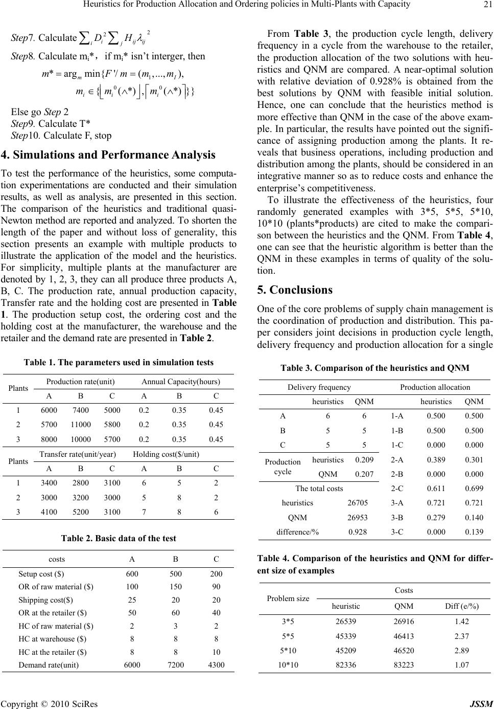

Heuristics for Production Allocation and Ordering policies in Multi-Plants with Capacity 21
Step7. Calculate2
2
iijij
ij
DH


Step8. Calculate mi*，if mi* isn’t interger, then
1
00
*arg min{'/(,...,),
{(*),(*) }}
mI
iii
mFmmm
mmm


 

Else go Step 2
Step9. Calculate T*
Step10. Calculate F, stop
4. Simulations and Performance Analysis
To test the performance of the heuristics, some computa-
tion experimentations are conducted and their simulation
results, as well as analysis, are presented in this section.
The comparison of the heuristics and traditional quasi-
Newton method are reported and analyzed. To shorten th e
length of the paper and without loss of generality, this
section presents an example with multiple products to
illustrate the application of the model and the heuristics.
For simplicity, multiple plants at the manufacturer are
denoted by 1, 2, 3, they can all produce three products A,
B, C. The production rate, annual production capacity,
Transfer rate and the ho lding cost are presented in Table
1. The production setup cost, the ordering cost and the
holding cost at the manufacturer, the warehouse and the
retailer and the demand rate are presented in Table 2.
Table 1. The parameters used in simulation tests
Production rate(unit) Annual C apacity(hours)
Plants A B C A B C
1 6000 7400 5000 0.2 0.35 0.45
2 5700 11000 5800 0.2 0.35 0.45
3 8000 10000 5700 0.2 0.35 0.45
Transfer rate(unit/year) Holding cost($/unit)
Plants A B C A B C
1 3400 2800 3100 6 5 2
2 3000 3200 3000 5 8 2
3 4100 5200 3100 7 8 6
Table 2. Basic data of the test
costs A B C
Setup cost ($) 600 500 200
OR of raw material ($) 100 150 90
Shipping cost($) 25 20 20
OR at the retailer ($) 50 60 40
HC of raw material ($) 2 3 2
HC at warehouse ($) 8 8 8
HC at the retailer ($) 8 8 10
Demand rate(unit) 6000 7200 4300
From Table 3, the production cycle length, delivery
frequency in a cycle from the warehouse to the retailer,
the production allocation of the two solutions with heu-
ristics and QNM are compared. A near-optimal solution
with relative deviation of 0.928% is obtained from the
best solutions by QNM with feasible initial solution.
Hence, one can conclude that the heuristics method is
more effective than QNM in the case of the above exam-
ple. In particular, the results have pointed out the signifi-
cance of assigning production among the plants. It re-
veals that business operations, including production and
distribution among the plants, should be considered in an
integrative manner so as to reduce costs and enhance the
enterprise’s competitiveness.
To illustrate the effectiveness of the heuristics, four
randomly generated examples with 3*5, 5*5, 5*10,
10*10 (plants*products) are cited to make the compari-
son between the heuristics and the QNM. From Table 4,
one can see that the heuristic algorithm is better than the
QNM in these examples in terms of quality of the solu-
tion.
5. Conclusions
One of the core problems of supply chain management is
the coordination of production and distribution. This pa-
per considers joint decisions in production cycle length,
delivery freq uency and production allocation for a single
Table 3. Comparison of the heuristics and QNM
Delivery frequency Prod uction allocation
heuristicsQNM heuristicsQNM
A 6 6 1-A 0.500 0.500
B 5 5 1-B 0.500 0.500
C 5 5 1-C 0.000 0.000
heuristics0.209 2-A 0.389 0.301
Production
cycle QNM 0.207 2-B 0.000 0.000
The total costs 2- C 0 .611 0.699
heuristics 26705 3-A 0.721 0.721
QNM 26953 3-B 0.279 0.140
difference/% 0.928 3-C 0.000 0.139
Table 4. Comparison of the heuristics and QNM for differ-
ent size of examples
Costs
Problem sizeheuristic QNM Diff (e/%)
3*5 26539 26916 1.42
5*5 45339 46413 2.37
5*10 45209 46520 2.89
10*10 82336 83223 1.07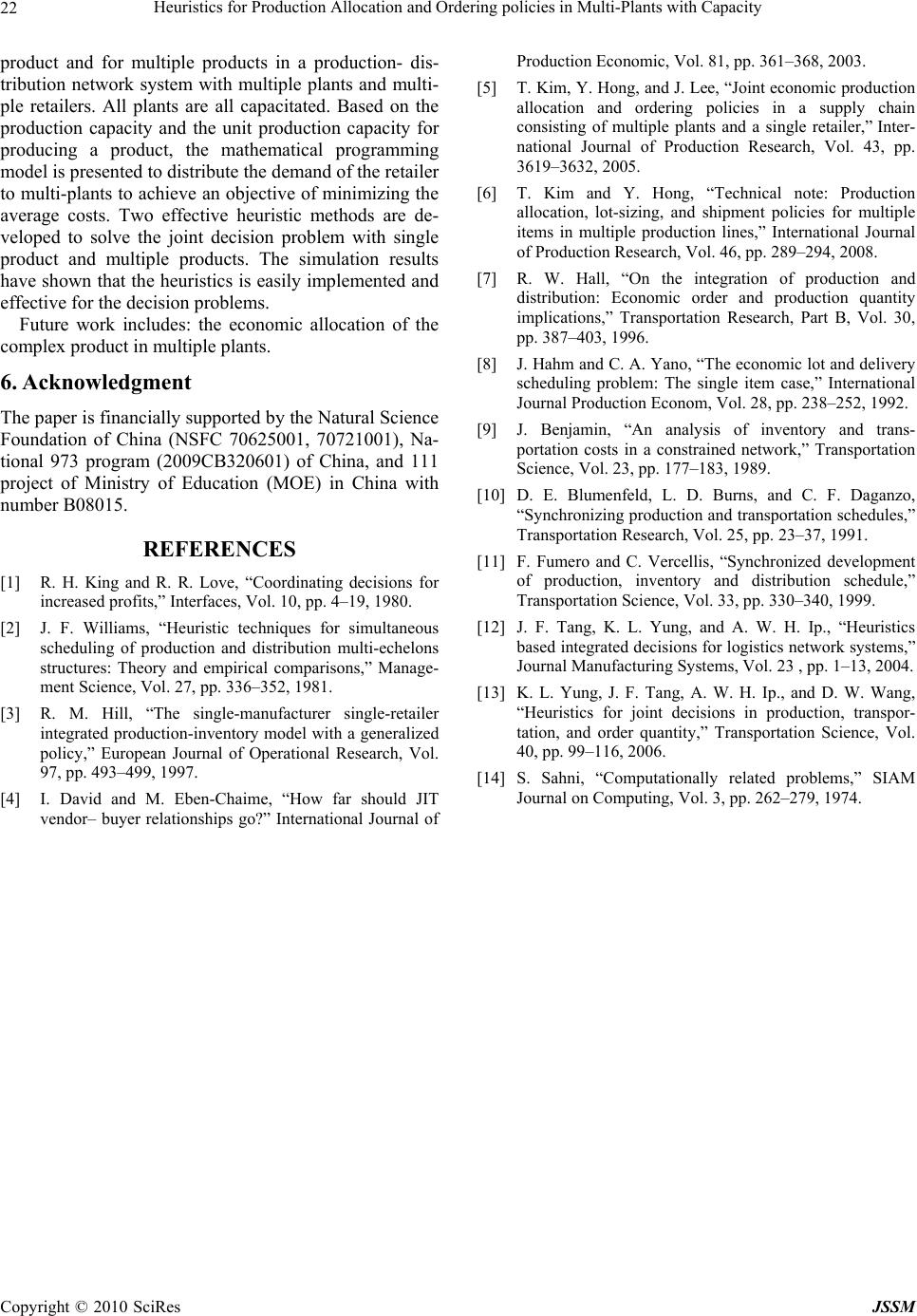

Heuristics for Production Allocation and Ordering policies in Multi-Plants with Capacity 22
product and for multiple products in a production- dis-
tribution network system with multiple plants and multi-
ple retailers. All plants are all capacitated. Based on the
production capacity and the unit production capacity for
producing a product, the mathematical programming
model is presented to distribute the demand of the retailer
to multi-plants to ach ieve an objective of minimizing the
average costs. Two effective heuristic methods are de-
veloped to solve the joint decision problem with single
product and multiple products. The simulation results
have shown that the heuristics is easily imple mented and
effective for the decision problems.
Future work includes: the economic allocation of the
complex product in multiple plants.
6. Acknowledgment
The paper is financ ially supported by the Natu ral Scienc e
Foundation of China (NSFC 70625001, 70721001), Na-
tional 973 program (2009CB320601) of China, and 111
project of Ministry of Education (MOE) in China with
number B08015.
REFERENCES
[1] R. H. King and R. R. Love, “Coordinating decisions for
increased profits,” Interfaces, Vol. 10, pp. 4–19, 1980.
[2] J. F. Williams, “Heuristic techniques for simultaneous
scheduling of production and distribution multi-echelons
structures: Theory and empirical comparisons,” Manage-
ment Science, Vol. 27, pp. 336–352, 1981.
[3] R. M. Hill, “The single-manufacturer single-retailer
integrated production-inventory model with a generalized
policy,” European Journal of Operational Research, Vol.
97, pp. 493–499, 1997.
[4] I. David and M. Eben-Chaime, “How far should JIT
vendor– buyer relationships go?” International Journal of
Production Economic, Vol. 81, pp. 361–368, 2003.
[5] T. Kim, Y. Hong, and J. Lee, “Joint economic production
allocation and ordering policies in a supply chain
consisting of multiple plants and a single retailer,” Inter-
national Journal of Production Research, Vol. 43, pp.
3619–3632, 2005.
[6] T. Kim and Y. Hong, “Technical note: Production
allocation, lot-sizing, and shipment policies for multiple
items in multiple production lines,” International Journal
of Production Research, Vol. 46, pp. 289–294, 2008.
[7] R. W. Hall, “On the integration of production and
distribution: Economic order and production quantity
implications,” Transportation Research, Part B, Vol. 30,
pp. 387–403, 1996.
[8] J. Hahm and C. A. Yano, “The economic lot and delivery
scheduling problem: The single item case,” International
Journal Production Econom, Vol. 28, pp. 238–252, 1992.
[9] J. Benjamin, “An analysis of inventory and trans-
portation costs in a constrained network,” Transportation
Science, Vol. 23, pp. 177–183, 1989.
[10] D. E. Blumenfeld, L. D. Burns, and C. F. Daganzo,
“Synchronizing production and transportation schedules,”
Transportation Research, Vol. 25, pp. 23–37, 1991.
[11] F. Fumero and C. Vercellis, “Synchronized development
of production, inventory and distribution schedule,”
Transportation Science, Vol. 33, pp. 330–340, 1999.
[12] J. F. Tang, K. L. Yung, and A. W. H. Ip., “Heuristics
based integrated decisions for logistics network systems,”
Journal Manufacturing Systems, Vol. 23 , pp. 1–13, 2004.
[13] K. L. Yung, J. F. Tang, A. W. H. Ip., and D. W. Wang,
“Heuristics for joint decisions in production, transpor-
tation, and order quantity,” Transportation Science, Vol.
40, pp. 99–116, 2006.
[14] S. Sahni, “Computationally related problems,” SIAM
Journal on Computing, Vol. 3, pp. 262–279, 1974.