Bayesian analysis of minimal model under the insulin-modified IVGTT

doi:10.4236/health.2010.23027

Paper Menu >>

Journal Menu >>

Vol.2, No.3, 188-194 (2010)

doi:10.4236/health.2010.23027

Health

Bayesian analysis of minimal model under the

insulin-modified IVGTT

Yi Wang1, Kent M. Eskridge2, Andrzej T. Galecki3

1,2Department of Statistics, University of Nebraska-Lincoln, Nebraska, USA

3Institute of Gerontology, University of Michigan, Michigan, USA

Received 24 September 2009; revised 23 October 2009; accepted 26 October 2009.

ABSTRACT

A Bayesian analysis of the minimal model was

proposed where both glucose and insulin were

analyzed simultaneously under the insulin-mo-

dified intravenous glucose tolerance test (IVG-

TT). The resulting model was implemented with

a nonlinear mixed-effects modeling setup using

ordinary differential equations (ODEs), which

leads to precise estimation of population pa-

rameters by separating the inter- and intra-indi-

vidual variability. The results indicated that the

Bayesian method applied to the glucose-insulin

minimal model provided a satisfactory solution

with accurate parameter estimates which were

numerically stable since the Bayesian method

did not require ap proximation by linearization.

Keywords: Minimal Model; Bayesian Analysis;

IVGTT; Nonlinear Mixed-Effects Modeling; ODE

1. INTRODUCTION

Mixed-ef fect s m odels that i nclude bo th fi xed and ra ndom

effects to account for the inter-individual variability are

becoming increasingly popular for analysis of population

pharmacokinetic/pharmacodynamic (PK/PD) data [1-8,

among others]. In these models it is assumed that all

responses follow a similar functional form, but that pa-

rameters vary a mong indivi du als. By separat ing the i nter-

and intra-individual variability , mixed-effects m odels will

often lead to more precise estimation of population pa-

rameters. Continuous pharmacokinetic processes are

often described by systems of ordinary differential equa-

tions (ODE) which generally lead to models that are

nonlinear in the parameters complicating estimation.

However, closed form solutions for systems of differen-

tial equations are not always possible therefore num erical

solutions of differential equations are necessary in order

to deal with many types of population PK/PD problems.

The nlmeODE in R given by Tornoe et al. [9] and

NLINMIX with ODE in SAS presented by Galecki et al.

[10], which can handle the first-order ODE’s by com-

bining odesolve with the NLME and NLINMIX respec-

tively, are used for parameter estimation in nonlinear

mixed-effects models. In addition, WBDiff (WinBUGS

Differential Interface) given by Lunn [11] is a useful tool

for dealing with pharmacokinetic models defined by

ODEs in the Bayesian setting. The analysis based on

ODEs may offer practical benefits in terms of easier

PK/PD modeling, particularly when more complicated

mechanistic models are used [12].

Diabetes is associated with a large number of abnor-

malities in insulin metabo lism, ranging from an absolute

deficiency to a combination of deficiency and resistance,

causing an inability to dispose glucose from the blood

stream. Three factors: Insulin sensitivity, Glucose effec-

tiveness, and Pancreatic responsiveness, referred to in

Pacini and Bergman [13], play an important role for

glucose disposal. Failure in any of these may lead to

impaired glucose tolerance, or, if severe, diabetes. Quan-

titative assessment is possible by the minimal model [14],

and may improve classification, prognosi s and therapy of

the disease. The minimal model is based on an intrave-

nous glucose tolerance test (IVG TT), where g lucose and

insulin concentrations in plasma are sampled after an

intravenous glucose injection. In patients with impaired

glucose tolerant (IGT), the insulin response to glucose

may be partially or totally suppressed. Of course, without

the insulin response, the glucose disappearance model

cannot provide an estimate of the metabolic parameters,

since there is no input to the model. The insulin modifi-

cation of IVGTT addressed the early problems with the

minimal model ‘failures’ by insulin injection at 20 min-

utes after glucose injection is given at time zero. Tradi-

tionally, in the minimal model the glucose and insulin

kinetics are described by two components, where the

parameters traditionally have been estimated separately

within each component by a nonlinear weighted least

squares estim ation tec hnique in a t wo-step pr ocedure [13].

The use of population an alysis to extract all information,

such as inter-subject variability, from experimental data

Y. Wang et al. / HEALTH 2 (2010) 188-194

189

brings about an improvement in the estimates of popula-

tion and individual characteristics. Previous work with

the IVGTT focused only on glucose kinetics where insu-

lin is treated as a known with no measurement errors for

non-Bayesian analysis [10] and for Bayesian analysis

[15]. However, the glucose-insulin system is an inte-

grated system and could be considered as a whole. An

assumption of the minimal model is that glucose and

insulin constitute a single dynamical system and impor-

tant information is lost in treating the insulin as known.

For example, pancreatic responsiveness, one important

factor of the individual metabolic portrait, cannot be

estimated if insulin is treated as known. Therefore, a

Bayesian analysis was adopted in combination with

population mixed-effects modeling to estimate the four

population and individual metabolic indices simultane-

ously with the minimal model of glucose and insulin

kinetics using data collected during insulin-modified

intravenous glucose tolerance test (IVGTT). No other

published wor k wa s ide nti fied t hat a naly zed bot h gluc ose

and insulin simultaneously under the insulin-modified

IVGTT.

2. METHODS

2.1. Bayesian Computational Algorithm for

WBDiff

Bayesian inference in WBDiff, which allows the nu-

merical solution of arbitrary systems of ODEs within

WinBUGS nonlinear mixed models, can be described

based on the followin g hierarchical modeling.

1) Suppose a chemical or pharmacokinetic model is

given by the systems of first-order ODE’s with the form

),,(/),(



txgdttdx , , , (1)

)(),( 00



xtx 0

tt

where x is an k-dimensional dependent variable vector, g

is the structural model while



is a q-dimensi onal vector

of unknown model parameters.

2) In nonlinear mixed-effects modeling, the within-

group variability describing the difference between the

observed response value and the predicted value can be

modeled as

~[() (,,);]

ijijiji ij

yNEyfx t









(2)

where i=1, m subjects and j=1, ni time points; is the

solution of Eq.1 and the relationship between the ob-

served response y and the predicted variable x is desig-

nated by a nonl i near function f.

3) The between-subject variability can be constructed

by defining the subject-specific random effects as

),(~ 





pi MVN (3)

where



is a vector of mean population ph armacok inetic

parameters and



is the variance-covariance matrix of

between-subj ect random variability.

4) In addition, hierarchical modeling in a Bayesian

setting comprises the prior specification, where prior

distributions are assigned to





, and



. For instance,



~MVNq(







-1~Wishartp(R,





~Gamma(a, b) (4)

The Bayesian inference is based on the following

principle: posterior  prior x likelihood. That is, the

so-called “likelihood function” is used to update “prior

beliefs” about some unknown parameters of interest to

“posterior beliefs” in the light of observed data. To obtain

the posterior estimators, using Monte Carlo approxima-

tion we simulate values from the joint posterio r distribu-

tion of all the model parameters given the observed data,

more specifically, the full conditional distribution. For

example, the logarithm of the full conditional distribution

for the random effect



i can be constructed as follows:





jiijii

iyfff 11 ),|(log),|(log)|(log



log||( )( )











log((, , ))

ijiji ij

nyfx t









 (5)

where the dot notation in denotes the distribution



i conditional upon everything else in the model. The

term

)|( 



),|(log







f refers to the logarithm of the prior

distribution for



i and this is specified to be a multivariate

normal distribution with mean vector θ and variance

-covariance matrix



. The term ),|(log





iij

,(iij

refers to

the log-likelihood of the jth observation fo r subject i under

the model, and the concentration yij was assumed to fol-

low a normal distribution with mean ), ij



and

variance



-1. Since we do not have a closed form for xij

from Eq.1, the numerical solution xij has to be obtained

from Eq.1 by fixing all the conditioning parameters so

that the Gibbs sampler can generate a new value, say



i(1)

from the full conditional distribution (Eq.5) given the

initial values to each unknown parameters



(0),



(0), and



(0). After n such iterations, the algorithm yields a joint

sample



i(n), which can be used for statistical inference in

WBDiff. The full conditional distributions for the other

model par ame ters can be co nstru cted i n a si mi lar m anner.

2.2. Population Analysis on Glucose-Insulin

Minimal Model

In this section, Bayesian analysis in combination with

population mixed-effects modeling was used to simulta-

neously estimate the four population and individual

metabolic indices: insulin sensitivity (SI), glucose effec-

tiveness (SG) and pancreatic responsiveness (



1 and



2),

based on the integrated glucose-insulin minimal model

Y. Wang et al. / HEALTH 2 (2010) 188-194

190

using data collected during the insulin-modified intra-

venous glucose tolerance test (IVGTT).

2.2.1. Bergman’s Modified Minimal Model

In an IVGTT study a dose of glucose was administered

intravenously over a 60 seconds period to overnight-

fasted subjects, 20 min after the glucose bolus, insulin

was injected over 1-2 min either into the portal vein or

into the femoral vein, and subsequently the glucose and

insulin concentrations in plasma were frequently sampled

(usually 30 ti mes) over a period of 180 minutes. Pr ofiles

of the 10 patients are displayed in Figure 1 [10].

Based on Figure 1, the intravenous glucose dose im-

mediately elevates the glucose concentration in the

plasma forcing the pancreatic β-cells to secrete insulin.

The insulin in the plasma is hereby increased, and the

glucose uptake in muscles, liver and tissue is raised by the

remote insulin in action. This lowers the glucose con-

centration in plasma, implying the β-cells to secrete less

insulin, from which a feedback effect arises [16]. The

integrate d gluc ose-ins ulin sy stem can be des cribe d by t he

following non-linearly coupled system of differential

equations, but this approach is not exactly the same model

as used in [17]. Here I1 is introduced to account for the

injection of insulin at t1 after the glucose bolus during the

IVGTT:

01 1

/(())()(),(0),

/( )(( )),(0)0,

/(())(()),(0),()

dGdtpG tGXt GtGG

dXdtp XtpItIX

dIdtn ItIG thtIIItI





 

  

 

(6)

where t=0 is the glucose injection time, + denotes posi-

tive reflection, namely,

() ,(),

(() )

0, .

Gt hGth

Gt h

otherwise



















and the model parameters are as explained in [13].

2.2.2. Bayesian Analysis of Bergman’s Modified

Minimal Model Using WBDiff

A Bayesian framework for modeling the time-varying

glucose and insulin profiles during the IVGTT and in-

ter-individual variability requires a three-stage hierar-

chical model. At the first stage, glucose values G(tj,θi)

and insulin values I(tj,θi) in subject i at time tj were ob-

tained as the solutions to Eq.6. The model we consider

assumes Gij = G(tj,θi) + εij1 and Iij = I(tj,θi) + εij2, where

εijk is a mean zero norm ally and independently distributed

error term. An additional assumption about within-

subject errors will be forthcoming in due course. Stacking

the two response variables Gij and Iij into a single re-

sponse vector, an indicator variable for the two res po nses

can be used to construct the model function. By combin-

ing G() and I(), we obtain

(, ),

ijkjiij

Yft









where (,),

ijij ij

YGI(, ),1

(, )

(, ),2

kji

Gt k

It k















and

θi is a vector of parameters of this model

for subject i denoted by

(, ).



ij ij





1230 011

(,, ,,,,,,,).

iiiiiiiiii i

pppGn hItI





Here it is further assumed that the time when insulin

injection occurs after glucose injection at time zero is also

an unknown parameter denoted as t1 which must be es-

timated. To account for correlation between the two re-

sponse variables m easured on the sam e occasion, we m ay

assume the elements of εij are correlated, with vari-

ance-covariance matrix τ-1



2. Here for simplicity it is

assumed that



2=I2, since the intent in this paper is to

introduce the random effects to account for in-

ter-individual variability rather than define a vari-

ance-covariance structure for random errors to address

intra-individual variability. However, the variance func-

tion fk2(tj,



) and the weight wj are specified for hetero-

geneous within-subject error (εijk) variance for two rea-

sons: 1) the glucose and insulin concentration points

before 8 minu tes can then be zero-weighted to account for

the time taken by the injected glucose to diffuse in its

distribution space, which can be ac hieved by setting wj=0

at any tim e points bef ore 8 minutes and wj=1 for others; 2)

it is commonly recognized that intra-subject variation of

this kind tends to increase with plasma concentration

level. That is, the higher the concentration level, the lar-

ger the variation so that less weight should be assigned.

Thus, we assume the following covariance matrix for the

within-subject errors εijk.

230

(,) 0

|~ 0,



 





































































The second stage is characterized by making assump-

tions about individual parameters. In particular, it was

assumed that the individual parameters were drawn from

a multivariate log-normal distribution guaranteeing non-

negativity of parameters

1230 0111010

(,,,,,,,,, )~(,),

iiiiiiiii ix

pppGnh ItILnormal





where



is an unknown population mean vector and



is an unknown covariance matrix. At the third stage, prior

distributions for population parameters





, and τ were

specified. These prior distributions were vague repre-

senting a ‘lack’ of prior knowledge with:

Y. Wang et al. / HEALTH 2 (2010) 188-194

191

Figur e 1. Individual glucose and insulin profiles for 10 patients.

was the mean for



derived from nonl inear wei ghted least

squares minimization on

410

~[,10NormalI ],



~Gamma

110

~[10,0.01Wishart I





(0.001,0.001), ],



where })),(()),({( 2

2ijij

jijijijtIItGGw





 



ˆ(3.5, 4.6, 10,1.35, 5.8,4.4,5.6,5.9,5.8,3)T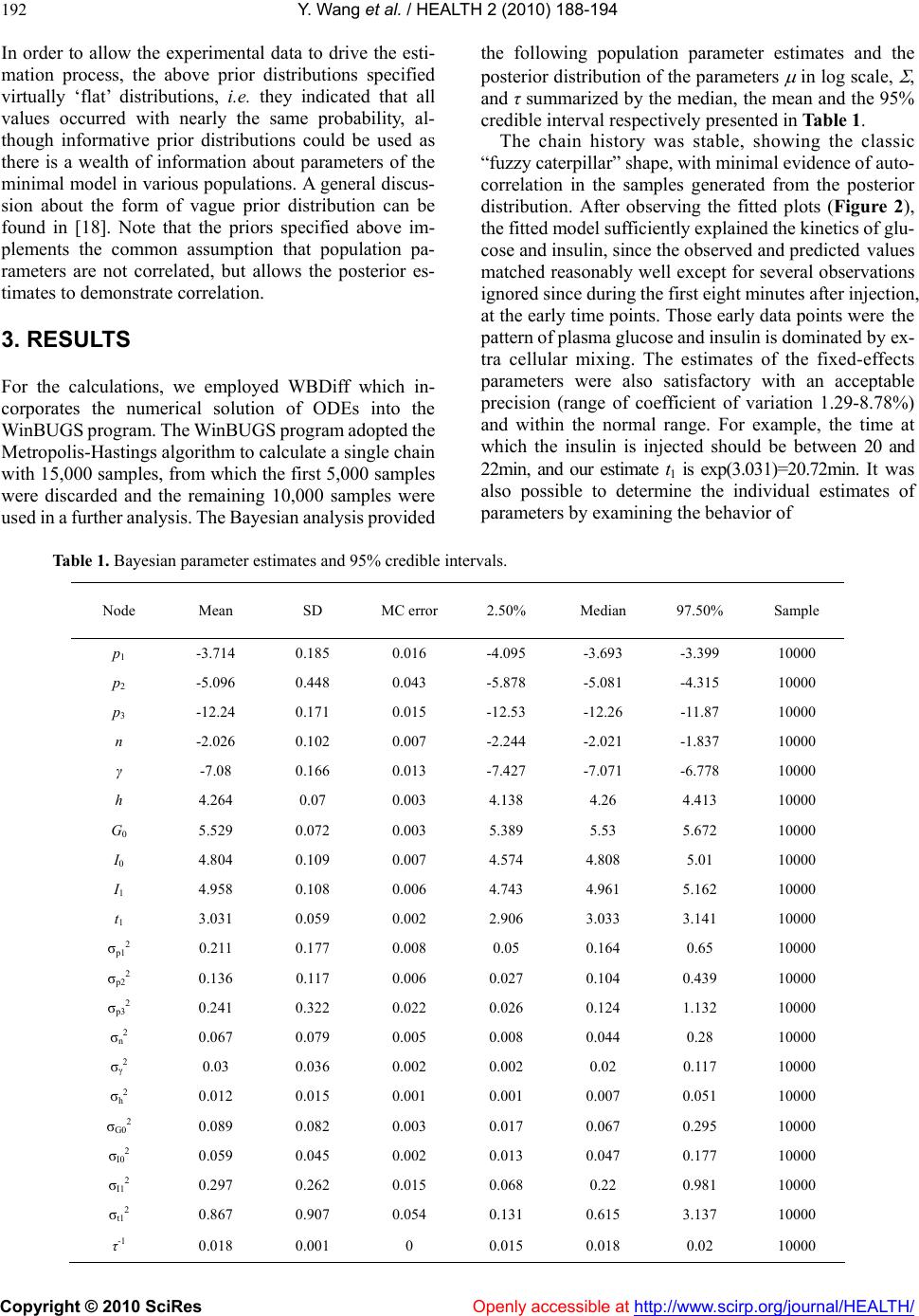



 

Y. Wang et al. / HEALTH 2 (2010) 188-194

192

In order to allow the experimental data to drive the esti-

mation process, the above prior distributions specified

virtually ‘flat’ distributions, i.e. they indicated that all

values occurred with nearly the same probability, al-

though informative prior distributions could be used as

there is a wealth of information about parameters of the

minimal model in v arious populations. A general discus-

sion about the form of vague prior distribution can be

found in [18]. Note that the priors specified above im-

plements the common assumption that population pa-

rameters are not correlated, but allows the posterior es-

timates to demonstrate correlation.

3. RESULTS

For the calculations, we employed WBDiff which in-

corporates the numerical solution of ODEs into the

W inBUGS program. The W inBUGS program adopted the

Metropolis-Hastings algorithm to calculate a single chain

with 15,000 samples, from which the first 5,000 samples

were discarded and the remaining 10,000 samples were

used in a further analysis. The Bayesian analysis provided

the following population parameter estimates and the

posterior distr ibution of the parameters



in log scale,



and τ summarized by the median, the mean and the 95%

credible interval respectively presented in Table 1.

The chain history was stable, showing the classic

“fuzzy caterpillar” shape, with minimal evidence of auto-

correlation in the samples generated from the posterior

distribution. After observing the fitted plots (Figure 2),

the fitted model sufficiently explained the kinetics of glu-

cose and insulin, since the observed and predicted values

matched reasonably well except for several observations

ignored since during the first eight minutes after injection,

at the early time points. Those early data points were the

pattern of plasma gluc ose and i nsulin is dominated by ex-

tra cellular mixing. The estimates of the fixed-effects

parameters were also satisfactory with an acceptable

precision (range of coefficient of variation 1.29-8.78%)

and within the normal range. For example, the time at

which the insulin is injected should be between 20 and

22min, and our estimate t1 is exp(3.031)=20.72min. It was

also possible to determine the individual estimates of

paramete rs by examining the behavi o r o f

Table 1. Bayesian parameter estimates and 95% credible intervals.

Node Mean SD MC error 2.50% Median 97.50% Sample

p1 -3.714 0.185 0.016 -4.095 -3.693 -3.399 10000

p2 -5.096 0.448 0.043 -5.878 -5.081 -4.315 10000

p3 -12.24 0.171 0.015 -12.53 -12.26 -11.87 10000

n -2.026 0.102 0.007 -2.244 -2.021 -1.837 10000

γ -7.08 0.166 0.013 -7.427 -7.071 -6.778 10000

h 4.264 0.07 0.003 4.138 4.26 4.413 10000

G0 5.529 0.072 0.003 5.389 5.53 5.672 10000

I0 4.804 0.109 0.007 4.574 4.808 5.01 10000

I1 4.958 0.108 0.006 4.743 4.961 5.162 10000

t1 3.031 0.059 0.002 2.906 3.033 3.141 10000

σp12 0.211 0.177 0.008 0.05 0.164 0.65 10000

σp22 0.136 0.117 0.006 0.027 0.104 0.439 10000

σp32 0.241 0.322 0.022 0.026 0.124 1.132 10000

σn2 0.067 0.079 0.005 0.008 0.044 0.28 10000

σγ2 0.03 0.036 0.002 0.002 0.02 0.117 10000

σh2 0.012 0.015 0.001 0.001 0.007 0.051 10000

σG02 0.089 0.082 0.003 0.017 0.067 0.295 10000

σI02 0.059 0.045 0.002 0.013 0.047 0.177 10000

σI12 0.297 0.262 0.015 0.068 0.22 0.981 10000

σt12 0.867 0.907 0.054 0.131 0.615 3.137 10000

τ-1 0.018 0.001 0 0.015 0.018 0.02 10000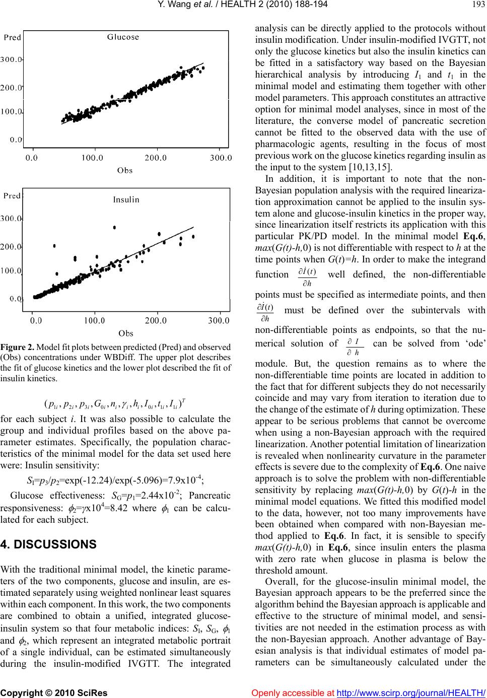

Y. Wang et al. / HEALTH 2 (2010) 188-194

193

Figure 2. Model fit plots between predicted (Pred) and observ ed

(Obs) concentrations under WBDiff. The upper plot describes

the fit of glucose kinetics and the lower plot described the fit of

insulin kinetics.

1230 011

(,,,,,,,,, )

iiiiiiiiii

pppGn hItI



for each subject i. It was also possible to calculate the

group and individual profiles based on the above pa-

rameter estimates. Specifically, the population charac-

teristics of the minimal model for the data set used here

were: Insulin sensitivity:

SI=p3/p2=exp(-12.24)/exp(-5.096) =7.9x10-4;

Glucose effectiveness: SG=p1=2.44x10-2; Pancreatic

responsiveness:



2=γx104=8.42 where



1 can be calcu-

lated for each subject.

4. DISCUSSIONS

With the traditional minimal model, the kinetic parame-

ters of the two components, glucose and insulin, are es-

timated separately using weighted nonlinear least squares

within each c omponent. In thi s work, the two com ponents

are combined to obtain a unified, integrated glucose-

insulin system so that four metabolic indices: SI, SG,



and



2, which represent an integrated metabolic portrait

of a single individual, can be estimated simultaneously

during the insulin-modified IVGTT. The integrated

analysis can be directly applied to the protocols without

insulin m odificat ion. Unde r insul in-m odifie d IVGT T, not

only the glucose kinetics but also the insulin kinetics can

be fitted in a satisfactory way based on the Bayesian

hierarchical analysis by introducing I1 and t1 in the

minimal model and estimating them together with other

model parameters. This approach constitutes an attractive

option for minimal model analyses, since in most of the

literature, the converse model of pancreatic secretion

cannot be fitted to the observed data with the use of

pharmacologic agents, resulting in the focus of most

previous wor k on the glucose ki netics regarding insulin as

the input to the system [10,13,15].

In addition, it is important to note that the non-

Bayesian population an alysis with the required lin eariza-

tion approximation cannot be applied to the insulin sys-

tem alone and glucose-insulin kinetics in the proper way,

since linearization itself restricts its application with th is

particular PK/PD model. In the minimal model Eq.6,

max(G(t)-h,0) is not differentiable with respect to h at the

time points when G(t)=h. In order to make the integrand

function ()



 well defined, the non-differentiable

points must be specified as intermediate points, and then

()



 must be defined over the subintervals with

non-differentiable points as endpoints, so that the nu-

merical solution of



can be solved from ‘ode’

module. But, the question remains as to where the

non-differentiable time points are located in addition to

the fact that for different subjects they do not necessarily

coincide and may vary from iteration to iteration due to

the change of the estim ate of h during optimization. These

appear to be serious problems that cannot be overcome

when using a non-Bayesian approach with the required

linearization. Another potential limitation of linearization

is revealed when nonlinearity curvature in the parameter

effects is se vere due to the com plexity of Eq.6. One naive

approach is to solve the problem with non-differentiable

sensitivity by replacing max(G(t)-h,0) by G(t)-h in the

minimal model equations. We fitted this modified model

to the data, however, not too many improvements have

been obtained when compared with non-Bayesian me-

thod applied to Eq.6. In fact, it is sensible to specify

max(G(t)-h,0) in Eq.6, since insulin enters the plasma

with zero rate when glucose in plasma is below the

threshold amount.

Overall, for the glucose-insulin minimal model, the

Bayesian approach appears to be the preferred since the

algorithm behind the Bayesian app roach is applicable and

effective to the structure of minimal model, and sensi-

tivities are not needed in the estimation process as with

the non-Bayesian approach. Another advantage of Bay-

esian analysis is that individual estimates of model pa-

rameters can be simultaneously calculated under the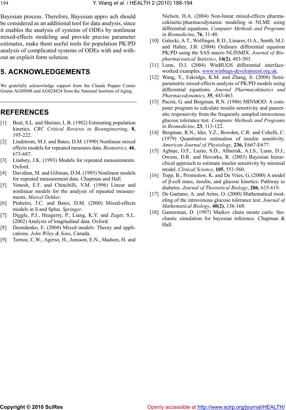

Y. Wang et al. / HEALTH 2 (2010) 188-194

194

Bayesian process. Therefore, Bayesian appro ach should

be considered as an additional tool for data a nalysis, since

it enables the analysis of systems of ODEs by nonlinear

mixed-effects modeling and provide precise parameter

estimates, make them useful tools for population PK/PD

analysis of complicated systems of ODEs with and with-

out an explicit form solution.

5. ACKNOWLEDGEMENTS

We gratefully acknowledge support from the Claude Pepper Center

Grants AG08808 and AG024824 from the National Institute of Aging.

REFERENCES

[1] Beal, S.L. and S heiner, L.B. (1982) Estimating population

kinetics. CRC Critical Reviews in Bioengineering, 8,

195-222.

[2] Lindstrom, M.J. and Bates, D.M . (1990) Nonlinear mixed

effects models for rep eated m easures data. Biometrics, 46,

673-687.

[3] Lindsey, J.K. (1993) Models for repeated measurements.

Oxford.

[4] Davidian, M. and Giltinan, D.M. (1995) Nonlinear models

for repeated measurement data. Chapman and Hall.

[5] Vonesh, E.F. and Chinchilli, V.M. (1996) Linear and

nonlinear models for the analysis of repeated measure-

ments. Marcel Dekker.

[6] Pinheiro, J.C. and Bates, D.M. (2000) Mixed-effects

models in S and Splus. Springer.

[7] Diggle, P.J., Heagerty, P., Liang, K.Y. and Zeger, S.L.

(2002) Analysis of longitudinal data. Oxford.

[8] Demidenko, E. (2004) Mixed models: Theory and appli-

cations. John Wiley & Sons, Canada.

[9] Tornoe, C.W., Agerso, H. , Jonsson, E.N., Madsen, H. and

Nielsen, H.A. (2004) Non-linear mixed-effects pharma-

cokinetic/pharmacodynamic modeling in NLME using

differential equations. Computer Methods and Programs

in Biomedicine, 76, 31-40.

[10] Galecki, A.T., Wolfinger, R.D., Linares, O.A ., Smith, M.J.

and Halter, J.B. (2004) Ordinary differential equation

PK/PD using the SAS mac ro NLINMIX. Journal of Bio-

pharmaceutical Statistics, 14(2), 483-503.

[11] Lunn, D.J. (2004) WinBUGS differential interface-

worked examples. www.winbugs-development.org.uk.

[12] Wang, Y., Eskridge, K.M. and Zhang, S. (2008) Semi-

parametric m ixe d-effects anal ysi s of PK /PD m odels u sing

differential equations. Journal Pharmacokinetics and

Pharmacodynamics, 35, 443-463.

[13] Pacini, G. and Bergman, R.N. (1986) MINMOD: A com-

puter program to calculate insulin sensitivity and pancre-

atic responsivity from the frequently sampled intravenous

glucose tolerance test. Computer Methods and Programs

in Biomedicine, 23, 113-122.

[14] Bergman, R.N., Ider, Y.Z., Bowden, C.R. and Cobelli, C.

(1979) Quantitative estimation of insulin sensitivity.

American Journal of Physiology, 236, E667-E677.

[15] Agbaje, O.F., Luzio, S.D., Albarrak, A.I.S., Lunn, D.J.,

Owens, D.R. and Hovorka, R. (2003) Bayesian hierar-

chical approach to estimate insulin sensitivity by minimal

model. Clinical Science, 105, 551-560.

[16] Topp, B., Promislow, K. and De Vries, G. (2000) A model

of β-cell mass, insulin, and glucose kinetics: Pathway to

diabetes. Journal of Theoretical Biology, 206, 615-619.

[17] De Gaetano, A. and Arino, O. (2000) Mathematical mod-

eling of the intravenous glucose tolerance test. Journal of

Mathematical Biology, 40(2), 136-168.

[18] Gamerman, D. (1997) Markov chain monte carlo: Sto-

chastic simulation for bayesian inference. Chapman &

Hall.
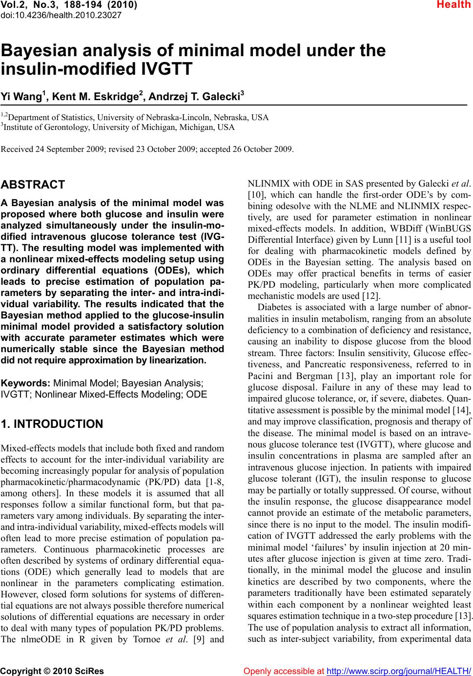