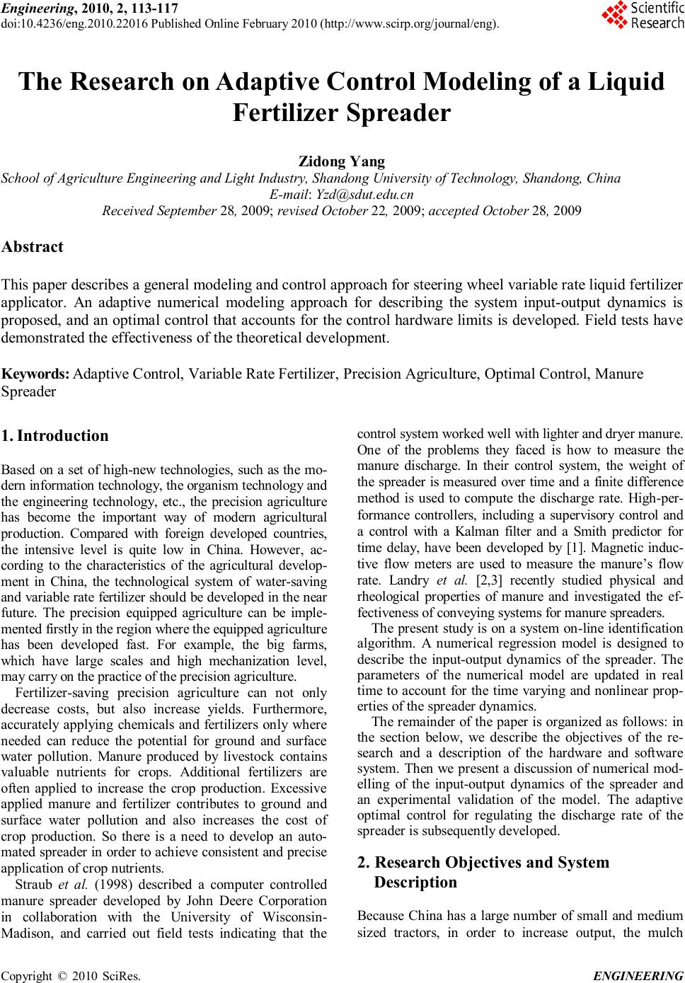Engineering, 2010, 2, 113-117
doi:10.4236/eng.2010.22016 Published Online February 2010 (http://www.scirp.org/journal/eng).
The Research on Adaptive Control Modeling of a Liquid
Fertilizer Spreader
Zidong Yang
School of Agriculture Engineering and Light Industry, Shandong University of Technology, Shandong, China
Received September 28, 2009; revised October 22, 2009; accepted October 28, 2009
Abstract
This paper describes a general modeling and control approach for steering wheel variable rate liquid fertilizer
applicator. An adaptive numerical modeling approach for describing the system input-output dynamics is
proposed, and an optimal control that accounts for the control hardware limits is developed. Field tests have
demonstrated the effectiveness of the theoretical development.
Keywords: Adaptive Control, Variable Rate Fertilizer, Precision Agriculture, Optimal Control, Manure
Spreader
1. Introduction
Based on a set of high-new technologies, such as the mo-
dern information technology, the organism technology and
the engineering technology, etc., the precision agriculture
has become the important way of modern agricultural
production. Compared with foreign developed countries,
the intensive level is quite low in China. However, ac-
cording to the characteristics of the agricultural develop-
ment in China, the technological system of water-saving
and variable rate fertilizer should be developed in the near
future. The precision equipped agriculture can be imple-
mented firstly in the region where the equipped agriculture
has been developed fast. For example, the big farms,
which have large scales and high mechanization level,
may carry on the practice of the precision agriculture.
Fertilizer-saving precision agriculture can not only
decrease costs, but also increase yields. Furthermore,
accurately applying chemicals and fertilizers only where
needed can reduce the potential for ground and surface
water pollution. Manure produced by livestock contains
valuable nutrients for crops. Additional fertilizers are
often applied to increase the crop production. Excessive
applied manure and fertilizer contributes to ground and
surface water pollution and also increases the cost of
crop production. So there is a need to develop an auto-
mated spreader in order to achieve consistent and precise
application of crop nutrients.
Straub et al. (1998) described a computer controlled
manure spreader developed by John Deere Corporation
in collaboration with the University of Wisconsin-
Madison, and carried out field tests indicating that the
control system worked well with lighter and dryer manure.
One of the problems they faced is how to measure the
manure discharge. In their control system, the weight of
the spreader is measured over time and a finite difference
method is used to compute the discharge rate. High-per-
formance controllers, including a supervisory control and
a control with a Kalman filter and a Smith predictor for
time delay, have been developed by [1]. Magnetic induc-
tive flow meters are used to measure the manure’s flow
rate. Landry et al. [2,3] recently studied physical and
rheological properties of manure and investigated the ef-
fectiveness of conveying systems for manure spreaders.
The present study is on a system on-line identification
algorithm. A numerical regression model is designed to
describe the input-output dynamics of the spreader. The
parameters of the numerical model are updated in real
time to account for the time varying and nonlinear prop-
erties of the spreader dynamics.
The remainder of the paper is organized as follows: in
the section below, we describe the objectives of the re-
search and a description of the hardware and software
system. Then we present a discussion of numerical mod-
elling of the input-output dynamics of the spreader and
an experimental validation of the model. The adaptive
optimal control for regulating the discharge rate of the
spreader is subsequently developed.
2. Research Objectives and System
Description
Because China has a large number of small and medium
sized tractors, in order to increase output, the mulch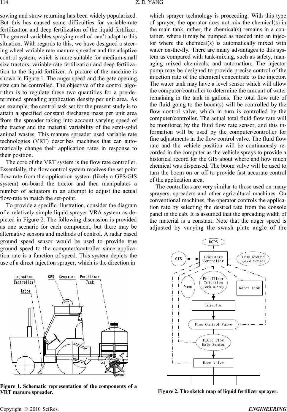

Z. D. YANG 114
sowing and straw returning has been widely popularized.
But this has caused some difficulties for variable-rate
fertilization and deep fertilization of the liquid fertilizer.
The general variables spraying method can’t adapt to this
situation. With regards to this, we have designed a steer-
ing wheel variable rate manure spreader and the adaptive
control system, which is more suitable for medium-small
size tractors, variable-rate fertilization and deep fertiliza-
tion to the liquid fertilizer. A picture of the machine is
shown in Figure 1. The auger speed and the gate opening
size can be controlled. The objective of the control algo-
rithm is to regulate these two quantities for a pre-de-
termined spreading application density per unit area. As
an example, the control task set for the present study is to
attain a specified constant discharge mass per unit area
from the spreader taking into account varying speed of
the tractor and the material variability of the semi-solid
animal wastes. This manure spreader used variable rate
technologies (VRT) describes machines that can auto-
matically change their application rates in response to
their position.
The core of the VRT system is the flow rate controller.
Essentially, the flow control system receives the set point
flow rate from the application system (likely a GPS/GIS
system) on-board the tractor and then manipulates a
number of actuators in an attempt to adjust the actual
flow-rate to match the set-point.
To provide a specific illustration, consider the diagram
of a relatively simple liquid sprayer VRA system as de-
picted in Figure 2. The following discussion is provided
as one scenario for each component, but there may be
alternative sensors and methods of control. A radar based
ground speed sensor would be used to provide true
ground speed to the computer/controller since applica-
tion rate is a function of speed. This system depicts the
use of a direct injection sprayer, which is the direction in
Figure 1. Schematic representation of the components of a
VRT manure spreader.
which sprayer technology is proceeding. With this type
of sprayer, the operator does not mix the chemical(s) in
the main tank, rather, the chemical(s) remains in a con-
tainer, where it may be pumped as needed into an injec-
tor where the chemical(s) is automatically mixed with
water on-the-fly. There are many advantages to this sys-
tem as compared with tank-mixing, such as safety, man-
aging mixed chemicals, and automation. The injector
pump may be designed to provide precise control of the
injection rate of the chemical concentrate to the injector.
The water tank may have a level sensor which will allow
the computer/controller to determine the amount of water
remaining in the tank in gallons. The total flow rate of
the fluid going to the boom(s) will be controlled by the
flow control valve, which in turn is controlled by the
computer/controller. The actual total fluid flow rate will
be monitored by the fluid flow rate sensor, and this in-
formation will be used by the computer/controller for
fine adjustments in the flow control valve. The fluid flow
rate and the vehicle position will be continuously re-
corded in the computer as the vehicle sprays to provide a
historical record for the GIS about where and how much
chemical was dispensed. The boom valve will be used to
turn the boom on or off to provide fast accurate control
of the application area.
The controllers are very similar to those used on many
sprayers, spreaders and other agricultural machines. On
conventional machines, the operator controls the applica-
tion rate by selecting the desired rate from the console
panel in the cab. It is assumed that the spreading width of
the material is a constant. Note that the auger speed is
adjusted by varying the swash plate angle of the
Figure 2. The sketch map of liquid fertilizer sprayer.

Z. D. YANG 115
hydraulic pump. In order to develop control algorithms to
achieve the above objective, we must first develop a dy-
namic model for the spreader. Specifically, we need a
relationship between the input, i.e. the auger speed and
the gate opening size, and the output, i.e. the material
discharge rate. Recall that the material is a highly inho-
mogeneous mix of liquids and solids with unknown per-
centage of each phase. The weight and viscosity of the
material affect the dynamics of the hydraulic system that
drives the auger. As the spreading proceeds, the amount
of material remaining in the tank changed. All these fac-
tors attribute to a nonlinear and time-varying dynamics of
the spreader. As discussed in Section 1, analytical mod-
eling of such a system is a difficult task. In this study, we
propose to develop an on-line numerical model of the
input-output relationship, known as the system transfer
function. The controller of on-line model has an Atmel
processor 89S51 with 33MHz frame rate. It communi-
cates with a laptop computer via RS232 at 9600 baud.
This controller can interface with and control a wide
range of equipment including variable rate applicators for
precision agriculture. The on-line system model fits the
experimental data to a pre-determined numerical model
with undetermined coefficients. A very common numeri-
cal model can describe a large.
3. On-Line System Modeling
Class of dynamic systems is the autoregressive model
with exogenous inputs (ARX) (Billings, 1986; Diaz and
Desrochers, 1988; Ljung, 1987). It is given in a general
form as
1(1)()
1()(1)
...
...
aa
kbkb
nnnnn
nnnnnn
yayay
bubu
−−
−−−+
+++
=++ (1)
The current output
n
y
is assumed to be a function of a
finite history of output values
(1)
n
y
−
to
()
a
nn
y− and the
delayed input
()
k
nn
u
− to
(1)
kb
nnn
u
−−+
. The coefficients
(1,...,)
ia
ain
=
and
(1,...,)
jb
bjn
=
are undetermined.
The on-line modeling algorithm determines the coeffi-
cients and approximates the numerical model to the
measured system dynamics in some optimal manner.
Strictly speaking, the ARX model is valid for linear
dynamic systems. The present spreader system is time
varying and nonlinear. A properly identified ARX model
will accurately represent the dynamics of the system over
a short time interval and will not be valid for the entire
history of the spreading task from a full tank to empty.
Therefore the ARX model must be updated frequently
during spreading. Efficient real-time adaptive algorithms
will be needed for this task.
3.1. Adaptive Algorithm
In signal processing, the ARX model is also known as an
infinite impulse response (IIR) filter (Haykin, 1991).A
popular steepest gradient descent method known as the
least mean square (LMS) algorithm (Widrow and Stearns,
1985) can be used to adjust the coefficients of the ARX
model and minimize the error between the prediction of
the numerical model and the real measurement. The es-
timation error is
kkk
edy
=−
, where
k
d
is the meas-
ured output and
k
y
is the predicted output. A perform-
ance index can be defined as
2
()
k
Jke
=
. We write the
ARX model in a vector notation as
T
kkk
ywu
=
rr
(2)
where
T
kk
w
r
is a vector consisting of the undetermined
coefficients at the kth time step and
k
u
r
is a vector con-
sisting of both the past history of
k
y
and the control
inputs. The LMS algorithm for updating the undeter-
mined coefficients in order to minimize
()
Jk
is given by
(1)
kkkk
wweu
β
+=+
rrr
(3)
where β is an adaptation gain parameter.
3.2. Experimental Validation of the LMS
Algorithm
We have selected a simple ARX model for the spreader
given by
1(1)2(1)3(1)
sg
kkkk
yayauau
−−−
=++ (4)
where
(1)
sk
u
−
denotes the swash plate angle that regulates
the auger speed and
(1)
g
k
u
−
is the rear gate opening. We
have carried out experiments to compare this simple
model with more complicated ones, and found that this
model describes the system with a good balance of accu-
racy and efficiency, and is sufficient for our work. A
digital second order IIR low pass filter of bandwidth 2Hz
programmed in the C language is used to block noise in
the weight signal. The weight signal is sampled at a rate
of 100 Hz in real time. During spreading, the gate posi-
tions are fixed for a period of time during which the
swash plate is swept from being completely closed to
being fully open to adjust the auger speed. The purpose of
doing so is to create a set of data from one test run that
excites as much of the system dynamics as possible. The
model prediction is seen to be quite accurate. The pa-
rameter a1 is nearly equal to one. This is physically rea-
sonable since in the absence of the control, i.e. when the
auger speed is zero and the gate is closed, the material
remaining in the tank is unchanged. The parameters a2
and a3 are negative. It is again physically reasonable that
a2 and a3 are negative. When the control inputs are
greater than zero, the material remaining in the tank yk
decreases. The ranges of these coefficients are as follows:

Z. D. YANG 116
max(a1)=1.0047, min(a1)=0.9881, average a1=1.0011;
max(a2)=−0.0083, min(a2)=−0.0111, averagea2=−0.0094;
max(a3)=−0.0045, min(a3)=−0.0080, average a3=−0.0063.
4. Control Algorithm
The control algorithm design depends on the system
model. This section focuses on a discussion of the con-
trol algorithm design. The integration of the control loop
and the parameter updating loop is natural and is coded
in the software.
4.1. Range Limited Optimal Control
Lewis and Syrmos [4] have shown that after going
through the steps of optimal control solutions and taking
i=k and N=k+1, we obtain the unconstrained optimal
control solution as
*1
1
()()
T
kkkkkk
uRccsNcsNaeG
−
=−++ (5)
We shall continue the study with the one step optimal
control. Recall that the range of
s
k
u
and
g
k
u
is finite.
The unconstrained optimal solution (5) is valid when the
bound is not exceeded. To account for the bounds on the
controls, we need to use the Pontryagin’s minimum prin-
ciple. This leads to the following in equality for deter-
mining the control
*
k
u
:
****
11
11
22
TTTT
kkkkkkkkkk
uRucuuRucu
λλ
++
+≤+ (6)
The inequality holds for all admissible values of
k
u
.
The optimal control can be found from the inequality by
considering an auxiliary problem of minimization of the
following quadratic form:
11
11
1
()()
2
T
kkkkkk
wuRcuRcλλ
−−
++
=++ (7)
It can be shown that the
k
u
that minimizes w also
minimizes the left hand size of the inequality (5). Let the
lower and upper bounds of the control be denoted
by
min
,
sg
k
u
and
max
,
sg
k
u
. Let
,
sg
k
u
denote the swash plate and
gate opening control elements of the vector in Equation 5,
i.e.:
,1.
1
[()()]
sgTsg
kkkkkk
uRccsNcsNaeG
−
=−++ (8)
After several algebraic steps, we obtain the range con-
strained optimal control as
minmin
max
maxmax
,,,
*,,,,,
,,,
,
,
,
sgsgsg
kkk
sgsgsgsgsg
kkkkk
sgsgsg
kkk
uUu
uUuUu
uUu
≤


=<<

≥


(9)
The middle branch of the solution is the same as that
in Equation 5. In other words, when the system operates
within the physical limits of the controls, the solution
given by Equation 5 is optimal. Note that when the num-
ber of inputs is greater than the number of outputs, the
matrix R cannot be zero, and has to be positive definite.
4.2. Rate Limited Optimal Control
The range limited optimal control problem implies that
the controls can be instantly switched from one level to
another. This is of course not realistic since a physical
device always takes a finite time to change and has in-
herent delays. When the controller requires the system to
change faster than the physical rate limit, rate saturation
occurs. To account for the rate limits, we once again in-
voke the Pontryagin’s minimum principle and consider
the increment
1
k
u
−
∆such that
11
kkk
uuu
−−
=+∆ as the
control variable. Applying the Pontryagin’s minimum
principle in terms of the control increment, we have an-
other inequality
*******
1111111
1111111
1
()()()
21
()()()
2
TT
kkkkkkkk
TT
kkkkkkkk
uuRuucuu
uuRuucuu
λ
λ
−−−−+−−
−−−−+−−
+∆+∆++∆
≤+∆+∆++∆
(10)
The optimal control increment can be found from the
inequality by considering an auxiliary problem of mini-
mization of the following quadratic form:
)()(
2
11
1
111
1
11 +
−
−−+
−
−−+∆+∆+= kkkk
T
kkkk cRuucRuuw λλ
(11)
Define an increment by using Equation 8 as
,,.
1
sgsgsg
kkk
UUU
−
∆=− (12)
By minimizing w with respect to
1
k
u
−
∆, we obtain the
optimal control increment as
,,
,max
*,
1,,,
max,max
||
sgn()||
sgsg
kikk
sg
k
sgsgsg
kkikk
UUu
uUuUu
−

∆∆≤∆

∆=

∆∆∆>∆

 (13)
where
max
,
sg
k
u
∆ denotes the physically allowable maxi-
mum rate of change of the swash plate and rear gate
controls over one sample interval. The top branch of the
solution matches the range limited optimal control and
the lower branch is the rate saturated control. By com-
bining Equations 5 and 13, we obtain the optimal con-
trol under both range and rate saturation limits. More
discussions of such optimal control problems can be
found in Kobs and Sun (1997).
5. Discussions and Conclusions
In order to attain the goal of saving fertilizer, cutting down
production cost and protecting environment, the liquid
fertilizer applicator was designed and tested in field trial
based on its advantages of non-dust, non-smog and reduc-
ing environment pollution during the process of produc-
tion, usage and transportation. The optimized working

Z. D. YANG 117
parameters by means of field trial were as follows: fertili-
zation depth of 60-100 mm, operation velocity of 1.3m/s
and pump working pressure of 0.36 MPa. Let DA denotes
the required mass per unit area (kg/m2). The spreading
width is 1.5 m. A relationship between the discharge rate
Dt per unit time (kg/s), the speed of the tractor v (m/s) and
DA can be found as )/(167.4 skgvDD At =. Since the dis-
charge rate is constant when the tractor speed is constant,
the material remaining in the tank is a linearly decreasing
function of time. The actual measurement is in good
agreement with the reference input. Note that there is
significant noise in the measurement due to vehicle dy-
namics and electronic disturbances. The low pass digital
filter designed for the weight sensor is quite effective in
reducing measurement noise.
We have presented a general modeling and control ap-
proach for precision agricultural applications by using a
SYF-2 manure spreader as an example. The numerical
input-output modeling approach can handle a wide range
of variations in manure materials and the complicated
nonlinear dynamics of the machine. The adaptive self-
tuning optimal control algorithm can cope with various
hardware limits. The theoretical development has been
validated by extensive experimental results. The present
approach provides a promising methodology for automat-
ing machines for precision agricultural applications.
6. Acknowledgments
This paper supported by National Key Technology R&D
Program during the 11th Five-Year Plan Period of China
(2006BAD11A17) and the visiting scholar project of
excellent young teachers of higher learning in Shandong
Province.
7. References
[1] A. Munack, E. Buning, H. Speckmann, “A high-perfor-
mance control system for spreading liquid manure,” Con-
trol Engineering Practice, Vol. 9, pp. 387– 391, 2001.
[2] H. Landry, C. Lague, and M. Roberge, “Physical and
rheological properties of manure products,” Applied Engi-
neering in Agriculture, Vol. 20, No. 3, pp. 277– 288, 2004.
[3] H. Landry, E. Piron, J. M. Agnew, C. Lague, M. Roberge,
“Performances of conveying systems for manure spread-
ers and effects of Hopper geometry on output flow,” Ap-
plied Engineering in Agriculture, Vol. 21, No. 2, pp.
159–166, 2005.
[4] F. L. Lewis, V. L. Syrmos, “Optimal control,” John
Wiley and Sons, Inc., New York, 1995.