Engineering
Vol.06 No.13(2014), Article ID:52690,19 pages
10.4236/eng.2014.613092
Friction Material Temperature Distribution and Thermal and Mechanical Contact Stress Analysis
Carlos Abilio Passos Travaglia, Luiz Carlos Rolim Lopes
PPGEM―Programa de Pós Gradução em Engenharia Metalúrgica, UFF, Volta Redonda, Brazil
Email: carlosabiliotravaglia@gmail.com, luiz.crolim@uol.com.br
Academic Editor: Zhiwei Zhang, Romax Technology Inc., USA
Copyright © 2014 by authors and Scientific Research Publishing Inc.
This work is licensed under the Creative Commons Attribution International License (CC BY).
http://creativecommons.org/licenses/by/4.0/


Received 24 September 2014; revised 23 October 2014; accepted 18 November 2014
ABSTRACT
In brake systems, where the components are exposed to mechanical and thermal loads, the numerical analysis is very helpful. The main function of the brake system is to control or reduce vehicle’s speed by transformation of kinetic and potential energy in thermal energy. Using finite element method and Abaqus application, the present work proposed a model to study the impact of these loads on the performance of a pneumatic S cam drum brake’s friction material. The model included the effects of the rivet process; brake torque and warming in one of the 17 t bus front brake lining. Areas where the stresses vary with considerable amplitudes during temperature increase and brake application were identified. Also, it was possible to compare results of the numerical model to vehicle’s experimental measurements and understand its proximity to real braking events. By the application of the methodology and using the numerical model, pro- posed in this work, it will be possible to contribute considerably for a more accurate design of the friction material, besides undertake a better selection of the sub-compounds which it is made of.
Keywords:
Brake System, Friction Material, Heat Flux, Simulation, Numerical Analysis

1. Introduction
During pneumatic brake system actuation, the vehicle’s driver, by application of the brake pedal valve [1] , makes pressurized air enters inside front and rear mechanical actuators, generating forces which will pull the brakes shoes and linings against the rotating drums [2] [3] . Brake torque is then, generated on drum’s internal surface, resulting angular deceleration of the vehicle’s wheels.
In a typical commercial vehicle application, brake system is actuated several times in a repetitive way [2] , re- sulting on heat generation and cyclic mechanical efforts on the components in contact, such as brake drums, brake shoes and brake linings.
Numerical works on the effects of mechanical loads on these components have been published by some au- thors, as described for instance, on reference [4] , where a numerical analysis was performed considering all components of drum brake assembly, except the rivets that fixes the lining on the shoes. Analysis of the braking thermal and mechanical effects specially studied on isolated isotropic components, like brake drum, was already also performed by some authors [5] . However, the consequence of both thermal and mechanical loads on fric- tion materials, numerically molded as a composite made with fibers, particles and polymeric resin, is still not very well understood [6] [7] .
Neglecting the wear, considering perfect contact between lining and drum during braking and using the energy conservation principle, in accordance to the references [8] -[11] , a computational model for mechanical and ther- mal stress analysis in friction materials can be used by engineers in order to define, for instance, details in its geometry that could make this kind of material to have better response during real vehicle’s application, reducing development time and optimizing the costs of prototype vehicle preparation and tests.
On the other hand, friction material subcomponents selection, including its quantity and relative volume, will also be easier to be determined, once known the effects of mechanical loads and temperature distribution on the whole composite.
In the present work, the thermal and mechanical effects, including de riveting process and the temperature increase due to successive braking actions, on the brake lining, are studied and presented. The friction material, in this work, was numerically molded as an orthotropic material (due to its manufacturing process) [7] , formed by glass “E-type” fibers solved into a Phenolic Resin matrix.
2. Material and Methods
In urban buses applications, where the brakes are applied with high frequency, the cooling intervals are not larger enough and the convective effect on the drums is not efficient, the temperature level can cause reduction of mechanical resistance, increase of wear and may provide considerable impact on the friction material stress distribution.
On Figure 1 it’s possible to observe failures on S cam drum brake friction material after accumulation of some mileage during bus application durability test.
Based on that, the subject of this work is to build and validate a numerical model that could help engineers to:
・ Correctly design (dimension and develop) brake’s friction material;
・ Understand thermo-mechanical phenomena on brakes in order to turn new composites development easier;
・ Understand mechanisms of failure on friction materials during durability tests after consecutive cycles of brake application.
The numerical model was built up with applicative Abaqus 6.12 and the input data was calculated based on field urban bus braking application experimental measurements.
2.1. Steps of the Work
Development of this work has consisted on the following steps (Figure 2).
2.2. Data Acquirement
A 17 t load capacity bus, equipped with S cam drum brakes has percussed a typical 23 km total extension urban route in Osasco, SP, Brazil. During this percuss driver has applied vehicle’s brake pedal several times in order to keep its velocity the same and stop at bus stations and transit lights, making the brakes to accumulate thermal energy until completing the whole route.
The total time of the route was approximately 2 hours (7200 s). During this time some data was acquired by special equipment:
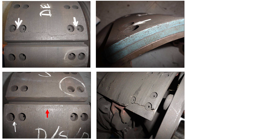
Figure 1. Damages on friction materials after durability tests.
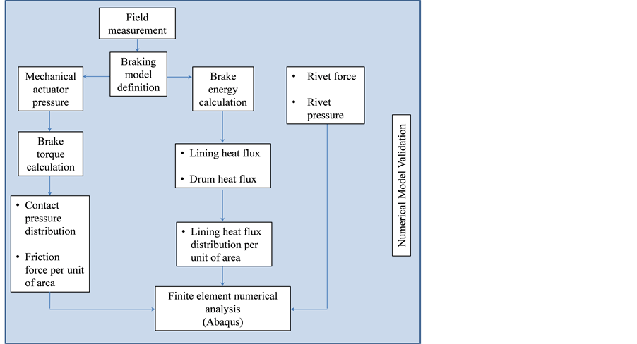
Figure 2. Activities of the project.
・ Vehicle’s velocity: v;
・ Vehicle’s altitude: h;
・ Pneumatic pressure inside front mechanical brake actuator: ;
;
・ Averaged temperature of front brake’s friction material: ;
;
・ Temperature of front brake’s friction film: T;
・ Environment temperature: .
.
The instant of highest actuator pressure and brake torque has occurred during a braking performed between 6935 s and 6965 s of vehicle’s percuss. During this interval, the friction film temperature, T, measured by ther- mocouple positioned 1 mm from the drum’s internal surface [2] [3] , has varied between 321˚C and 340˚C (Figure 3), and the averaged friction material temperature,  , measured by thermocouple positioned 5 mm from the friction surface of the lining, was approximately 280˚C. On Figure 3,
  and
and  denotes initial and final braking instants.
Variation of the vehicle’s linear velocity, v, and altitude, h, during this braking was also obtained. It’s presented on Figure 4 below, where i and f denotes respectively, initial and final braking instants.
3. Theory and Calculation
In this section, the basic theory applicable to the work is presented. Calculation of the data necessary for the numerical simulation and preparation of the model are also part of this section.
3.1. Theory of Braking
3.1.1. Brake Torque and Distribution of Contact Pressure during Braking
The maximum contact pressure on the friction material during the braking in S cam brakes is defined by the Equation (1), where W is the lining width and  is the Coulomb friction coefficient between surfaces in contact,
  is the lining surface radius and
 ,
,  e
e  defines specific wheel brake’s angular positions. It’s possible to verify on Equation (1) that the maximum contact pressure is proportional to the brake torque
  [12] :
 (1)
(1)
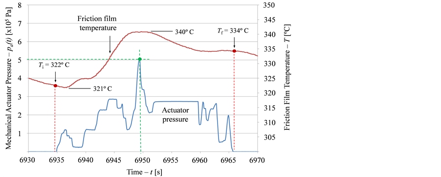
Figure 3. Actuator pressure and friction film temperature variation during high- est brake torque braking.
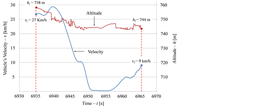
Figure 4. Vehicle’s velocity and altitude variation during highest brake torque braking.
The expressions  and
and  defines respectively initial and final angular positions of the friction material’s surface in contact with the drum. They can be expressed by
  and
and .
.
On the other hand, the brake torque,  , is defined by Equation (2), where BF, brake factor (relationship between friction and input forces
  and
and ),
),  , sectional area of the mechanical actuator,
  , length of the slack adjuster, and
 ,
,  cam’s effective radius, are geometrical parameters of the brake,
  is the mechanical efficiency and
  and
and , empirical factors. The brake torque is also proportional to the difference between pneumatic pressure inside mechanical actuator,
  and threshold pressure, p0 [2] :
 (2)
(2)
The angles ,
,  e
e , as well, brake’s geometrical parameters, can be observed on Figure 5.
The contact pressure on the friction material’s surface varies with the angular position,  and braking time,
  , defined within the intervals
  and
and , according to Equation (3) below [13] .
 (3)
(3)
It’s easy to observe that the maximum contact pressure will take place at .
.
3.1.2. Distribution of Friction Force per Unit of Area
Consider the drum brake system diagram defined on Figure 6 as follows:
The element of friction force,  can be described as function of Coulomb friction coefficient between lining and drum,
  , and the element of normal force,
 . On the other hand,
  can be describ- ed as function of the contact pressure,
  and the element of area,
 . Considering perfect contact between lining and drum [14] , it’s possible to define:
 (4)
(4)
After splitting both sides of Equation (4) by the element of area,  , it’s obtained:
 (5)
(5)
where: . (6)
. (6)
3.1.3. Braking Energy Generation and Heat Absorption
1) Mechanical Energy Conservation
The heat generated on the brakes can be calculated by the mechanical energy conservation principle. Neglecting optical, noise, particles pulverization and other forms of energy [14] [15] , the braking energy,  , can be expressed by:

Figure 5. S cam brake geometry.
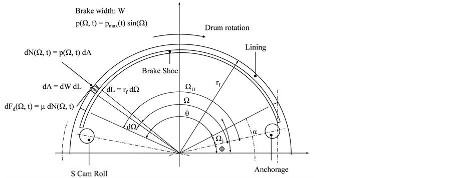
Figure 6. Drum brake system: Load diagram.
 (7)
(7)
where m is the vehicle mass, g is the local gravity acceleration and k is the rotational elements inertia factor. Typical values of k are between 1.03 and 1.60 [2] .
2) Energy Absorbed by the Brakes
The quantity of energy absorbed by the brake,  , is proportional to its participation over the braking,
  [2] [16] . Then it’s possible to define it generically according to:
 (8)
(8)
The averaged heat flux,  on the brake can be obtained by the braking time, t [2] [16] :
 (9)
(9)
Part of brake energy is absorbed by friction material and part by the drum. Based on the energy conservation principle and considering perfect contact, it’s possible to describe:
 (10)
(10)
where  denotes the averaged heat flux through the drum and
  denotes averaged heat flux through the lining.
  and
and  can be determined once known their respective thermal resistances,
  and
and  [2] :
[2] :
 (11)
(11)
In short braking events, the convective effect during brake’s actuation on both components can be neglected, then  and
and  can be expressed only as function of mass and thermal properties of drum and lining [2] :
 (12)
(12)
 (13)
(13)
where  is density,
  is specific heat and
  is thermal conductivity.
Once determined heat flux through friction material and drum, it’s possible to define the concept of energetic factor,  and
and , according to Equations (14) and (15) below:
 (14)
(14)
 (15)
(15)
3) Distribution of Friction Material’s Heat Flux per Unit of Area
The brake potency can be determined for each instant of the braking once known the brake torque,  and angular velocity of the wheel,
  , according to Equation (16) [2] [16] :
 (16)
(16)
Then, the instantaneous friction material’s heat flux can be calculated using the concept of energetic factor:
 (17)
(17)
The brake torque, function of time,  , is the sum of all friction force elements,
  multiplied by the brake radius,
 . As already shown, each element of friction force can be described as function of the con- tact pressure, element of area and friction coefficient between lining and drum. Considering two brake shoes per brake, it’s possible to define:
 (18)
(18)
That leads to:
 (19)
(19)
The friction material’s heat flux distribution per unit of area is obtained splitting Equation (19) by the element of area,  , where:
 (20)
(20)
Then, it’s defined, for one brake lining, in accordance with the references [17] [18] :
 (21)
(21)
where: . (22)
3.2. Determination of Data for the Numeric Model
3.2.1. Analytical Calculation: Brake Torque and Braking Energy
All data related to the brake design, vehicle’s characteristics and calculation of the loads can be found on the Appendix A.
3.2.2. Riveting Process Loads
The friction material is usually fixed on the brake shoe surface by rivets. The rivet process consists in applying an instantaneous peak of load on the rivets, making them to deform and compressing the joint components each other.
The peak of force on the rivets,  , was determined directly from the real manufacturing process. Table 1 specifies the efforts actuating on the rivets and their dimensional characteristics [3] . It was considered that the instantaneous pressure distribution on rivet’s extremities,
  , were uniform.
3.2.3. Friction Material Properties
It was assumed that the friction material was orthotropic with isotropy on the plans orthogonal to its manufacturing process compression direction [3] [6] [7] . This hypothesis has allowed to relation directional properties of the composite.
Table 2 presents some properties of the friction material. Some of them were calculated considering above mentioned hypothesis and assuming that this kind of composite is formed only by long glass E-type fibers solved into a Phenolic Resin matrix [3] [19] [20] .

Table 1. Rivet characteristics and loads.
Table 2. Friction material composition and properties.
3.3. Numerical Analysis
Numerical analysis of the braking was thermal coupled with mechanical (plan strain state). All the simulation was split in three steps, representing respectively the riveting process, the warming of the brakes until the begin- ning of the braking and the braking.
3.3.1. Simulation Steps
Before the steps, the initial temperature of the components, as well the model anchorage was defined. The initial temperature of lining, brake shoe and rivets were all set as environment, T∞ = 22˚C.
On the first step, the peak of pressure on the rivet’s heads and basis were applied. It was necessary to input the plasticity curve of the rivet material in the model (SAE 1020) [21] .
On the second step, the friction film temperature was fixed in 322˚C during all the time that preceded the braking (6935 s), establishing a heat flux through the brake components, making them to warm, up to the ther- mal equilibrium was attained.
The braking event was simulated on the third step.
3.3.2. Loads, Boundary Conditions and Properties
Figure 7 shows mechanical efforts and thermal load, as well, degrees of freedom, anchorages and polar coordi- nate system of the brake section defined for the study.
Before performing simulation, it was necessary to enter calculated data (Appendix A), to define material pro- perties: rivet, isotropic―SAE 1020; shoe, isotropic―EN-GJS-500-7 and friction material, orthotropic Table 2; besides material orientation, reference coordinate systems, convection surfaces, interface areas, etc.
The convective coefficient, h, has corresponded to the natural convection. Conductance between different com- ponents was compatible with the materials [3] [22] .
4. Results
After simulation, temperature distribution and most critical contact shear stresses were obtained. They are presented on the following sections.
4.1. Temperature Distribution
Temperature distribution are presented for both thermal equilibrium and braking steps.
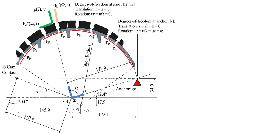
Figure 7. Mechanical efforts and thermal loads on the model.
4.1.1. Thermal Equilibrium (Step 2)
The minimum and maximum temperature of the assembly at the end of Step 2 were respectively 243˚C (516 K) and 319˚C (592 K). Figure 8 shows temperature distribution on the whole model after thermal equilibrium. The Figure 9 details the distribution on section AA (near to ) and the graphic of Figure 10 shows the temperature evolution in seven different radial positions.
4.1.2. Braking (Step 3)
During the braking, the hottest area of the friction material is near to the angular position  On the model, the temperature of the elements in this area reached about 356˚C during the maximum torque instant (t = 6949.50 s).
Figure 11 shows the temperature distribution during the maximum torque instant near to  and Figure 12 shows evolution of the friction material temperature during the braking in seven different radial positions.
It’s possible to observe on graphic of Figure 12, that the thermal effects of heat flux per unit of area, resulting of the contact between lining and drum during the braking, is not sensed by the elements and nodes in the proximity of the brake shoe. There was no temperature variation on lining elements located on the radius equal to 195 mm or lower (from 10 mm of the friction film).
4.2. Contact Shear Stresses
Figure 13 shows the four nodes of the model with highest magnitude of contact stresses. These nodes belong to the surface of friction material that supports the rivet’s heads.
The next graphics (Figure 14 and Figure 15) present variation of the contact shear stresses and temperature of these nodes during thermal equilibrium and braking steps.
All of these nodes have presented contact shear stresses with considerable magnitude variations, however, the highest amplitudes were verified on nodes 85,763 and 85,491, near to  (Figure 15).
During thermal equilibrium step, stress variation on node 85,763 due to temperature increase (from 22˚C to 255˚C) was 23.50 MPa. During this time it’s possible to verify inversion of the stress orientation around the node. The amplitude of contact stress during the braking was 9.30 MPa on the opposite orientation.
On the node 85,491 the contact stress variation during thermal equilibrium was 14.70 MPa. When the brakes were applied the stress was reduced in 12.70 MPa, showing that during braking application, there is also chang- ing of the contact shear stress orientation.

Figure 8. Temperature distribution on the model after thermal equilibrium.
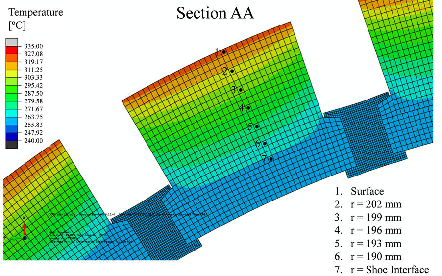
Figure 9. Temperature distribution on Section AA after thermal equilibrium.
4.3. Summary of the Results
Contact Shear Stress Analysis
Despite absent of a methodology acceptable for friction material fatigue resistance determination, it’s possible to
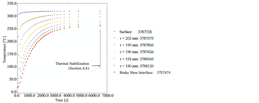
Figure 10. Temperature variation on Section AA during thermal equilibrium.
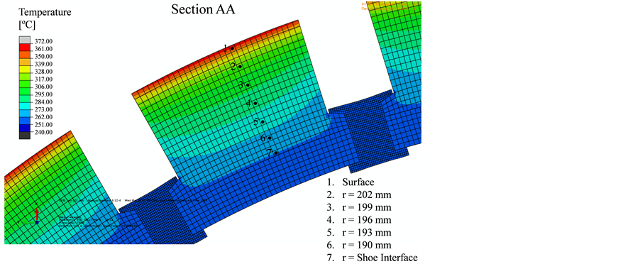
Figure 11. Temperature distribution on Section AA at maximum torque instant.
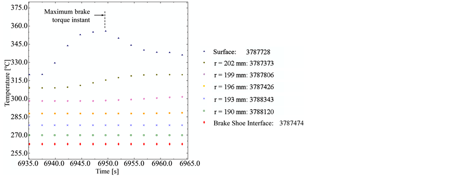
Figure 12. Temperature variation on Section AA during braking.
elaborate a hypothesis based on the numerical results.
After comparing the friction material of the vehicle’s front brakes after durability tests (Figure 1), where failure is associated to riveted regions, with the areas that presented highest contact shear stresses amplitudes on the
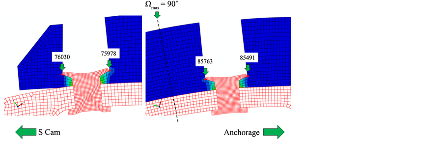
Figure 13. Nodes for contact shear stress analysis.
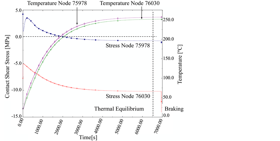
Figure 14. Variation of contact shear stress and temperature on nodes near to S cam-thermal equilibrium and braking.
numerical model (Figures 13-15), it was possible to associate the failures to accumulation of damage, due to cyclic contact stresses resulting from successive braking actions, on the interface between friction material and rivet.
The contact shear stresses at nodes 75,978 and 85,763 change in value and in sense, during the period of thermal equilibrium, as can be seen in Figure 14 and Figure 15 respectively. During braking action, some changes in value of the contact shear stresses are observed at all the four nodes, also according to Figure 14 and Figure 15. The most significant cyclic stress amplitude occurs in the proximity of .
.
The Table 3 below, shows the stresses amplitudes on nodes 76,030, 75,978 (near to S cam) and on nodes 85,763 and 85,491, near to  It’s easy to observe that the increase of assembly’s temperature (due to successive brake actuations) along vehicle’s percuss has caused more contact shear stress variation than the isolated effects of the braking event.
5. Numeric Model Validation
In this topic is presented a comparison between numerical results and experimental measurements performed on an urban bus with same type of brakes.
Figure 16 and Figure 17 show front brake shoe and friction material already prepared for the data acquirement.
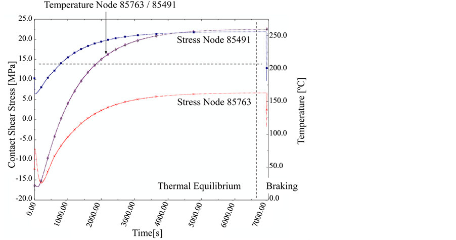
Figure 15. Variation of contact shear stress and temperature on nodes near to Ω = 90˚―Thermal equilibrium and braking.
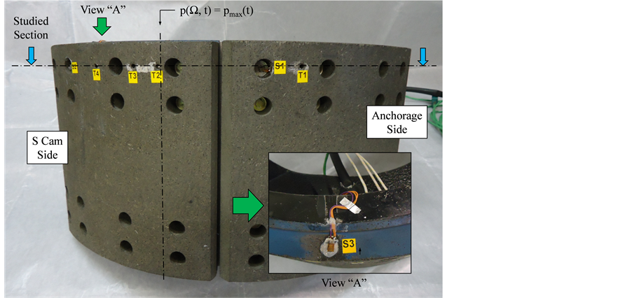
Figure 16. Brake shoe and friction material prepared for validation (upper side).
Table 3. Contact shear stresses amplitudes.
5.1. Friction Material Deformation
The experimental deformation was measured by two one-directional strain gages (S2 and S3) installed on the bus front brake friction material in different angular and radial positions (see Figure 16 and Figure 17) [3] . The data was obtained after one brake application (40 - 0 km/h) with brakes in cold condition (friction material temperature lower than 100˚C).
Figure 18 shows comparison between numerical and experimental deformation respectively on gages S2 and S3.
As it is possible to observe, experimental radial deformation along the time was in good agreement with numerical.
5.2. Friction Material Temperature Distribution
Temperatures were measured by thermo-couples ,
,  and
and , positioned in different angular and radial po- sitions inside the friction material:
  (r = 195 mm;
 ),
),  (r = 205 mm―friction film;
 ) and
) and  (r = 200 mm;
 ).
).
Experimental temperature distribution on front brakes was obtained after stabilization of the friction film
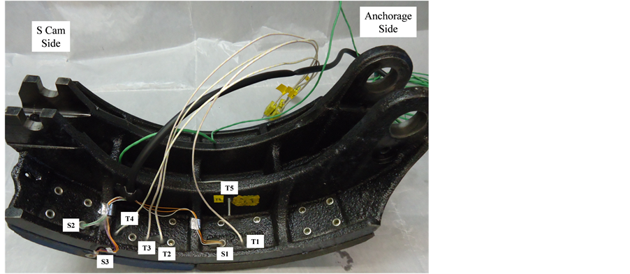
Figure 17. Brake shoe and friction material prepared for validation (down side).
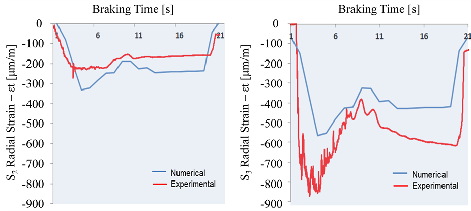
Figure 18. Comparison between experimental and numerical radial deformation of friction material (S2 and S3).
temperature [3] [23] . The test was performed on a special track. The temperature of the friction film of the front brakes has stabilized in 280˚C, after approximately 1500 s of the vehicle course.
Comparison between numerical and experimental temperature after stabilization shows a very good agreement. As can be observed on Figure 19, the largest difference between experimental and numerical data corresponds to the position of thermocouple T1 (stabilization temperatures were 237.80˚C and 248.30˚C respectively for experimental and numerical data).
5.3. Friction Film Temperature Variation
Comparison between numerical friction film temperature, obtained during simulation of the braking (Step 3) and experimental one, measured during the route of the bus in Osasco, SP (Figure 3) has shown relative good approach.
The error verified during maximum torque instant and at the end of the braking was respectively 4.20% and 0.30%, as can be seen on Figure 20.
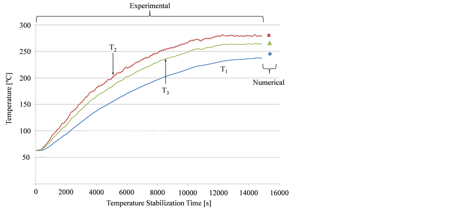
Figure 19. Friction material temperature distribution: Experimental × Numerical.
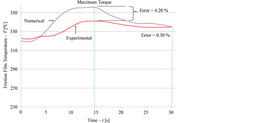
Figure 20. Friction film temperature comparison: Experimental × Numerical.
6. Conclusions
・ The main subject of the work, a numeric model and a methodology available and validated to be used by engineers, mentioned on Section 2, was attended because:
a. Critical areas, in terms of stress, identified on the model, have corresponded to areas where historically failures are observed during brake lining development tests. These stresses are related to the effects of the combination of thermal and mechanical load cycles on the surface contact between lining and rivets.
b. Numerical results are in good agreement with experimental data.
・ Friction material is vulnerable to cycling contact shear stresses on the interface between friction material and rivet’s head, mainly on the area with highest contact pressure, friction force and heat flux per unit of area . Combination of high brake torque amplitudes and elevated temperatures can be certainly harmful and drastically reduce the useful life of the friction materials.
・ With a friction material fatigue resistance limit determination methodology available, it is going to be possible to estimate the life of it, once the quantity of braking cycles and temperature are known. This will be feasible by adjusting the S x n curve by Goodman method and counting the damage cycles by rain flow technic [24] [25] .
・ Nodes where highest amplitudes of stresses were verified concur with vertices (intersection of rivet holes walls and the plans in contact with rivet’s heads). This means that improvements on brake lining geometry, such as, elimination of the vertices by cutting sharp edges, could be applied.
・ Numerical model presented, built with Abaqus applicative, will find practical application in the automotive industry in analysis related to brake’s system projects, including new friction materials development. The model will bring the following benefits:
a. The effects of the vehicle’s application brake temperature combined with brake torque loads on the friction material can be previously predicted without necessity of vehicle’s road tests. This will save development costs and time;
b. Assuming hypothesis that friction material is orthotropic, simulations using this model will contribute to design of the composite friction material and its composition;
c. Development of improved brake lining geometry and relative volume of the composite compounds.
・ As suggestion for next works, it’s highlighted.
a. Improvement of numerical model, including other components, like brake drum, S cam and brake’s anchors and rolls [2] [12] [13] .
b. Include variation of elastic properties of friction material with temperature.
c. Extend model to simulate effects of air convection through brake components during intervals between braking.
d. Include the effect of damage related to loss of lining materials resulting from brake action in the performance of the material in subsequent braking.
Acknowledgements
The authors are grateful to Smart-Tech for the discussions during development of the numerical model and out- put data analysis and to CAPES/MEC for the support to PPGEM/UFF.
References
- SAE International (2004) Bosch Automotive Handbook. 6th Edition, Warrendale, 800-801.
- Limpert, R. (1999) Brake Design and Safety. 2nd Edition, SAE International, Warrendale.
- Travaglia, C.A.P. (2014) Analise das Tensoes Termicas e Mecanicas no Material de Atrito de Veiculos Comerciais Equipados com Tambores de Freio Atraves do Metodo de Elementos Finitos. Mastering Thesis, Universidade Federal Fluminense, Volta Redonda.
- Hohmann, C., Schiffner, K., Oerter, K. and Reese, H. (1999) Contact Analysis for Drum Brakes and Disk Brakes Using ADINA. Computers & Structures, 72, 185-198. http://dx.doi.org/10.1016/S0045-7949(99)00007-3
- Amorim, G.B., Lopes, L.C.R., de Gouvêa, J.P., de Castro, J.A. and Tepedino, J.O.A. (2005) Determinação de Fadiga Termica em Tambores de Freio Atraves de Simulação Computacional. Proceedings of the 60th Annual ABM Inter- national Congress, Belo Horizonte, 25-28 July 2005, 1-10.
- Al-Qureshi, H.A. (1998) Composite Materials: Fabrication and Analysis. 3rd Edition, ITA, Sao Paulo.
- Casaril, A., Gomes, E.R., Soares, M.R., Fredel, M.C. and Al-qureshi, H.A. (2007) Análise Micro-mecânica dos Com- positos com Fibras Curtas e Partículas. Revista Matéria, 12, 408-419.
- Talati, F. and Jalalifar, S. (2009) Analysis of Heat Conduction in a Disk Brake System. Heat and Mass Transfer, 45, 1047-1059. http://dx.doi.org/10.1007/s00231-009-0476-y
- Shahril, K., Nordin, M. and Sulaiman, A.S. (2012) Temperature Analysis of Automotive Modeling Parts. Proceedings of the International Conference of Metallurgical, Manufacturing and Mechanical Engineering, Dubai, 26-27 December 2012, 285-288.
- Amorim, G.B., Lopes, L.C.R., de Gouvêa, J.P., de Castro, J.A. and Tepedino, J.O.A. (2005) Determinação de Ciclos Ter- micos Resultantes de Eventos de Frenagem em Tambores de Freio Atraves de Simulação Computacional. Proceedings of the 60th Annual ABM International Congress, Belo Horizonte, 25-28 July 2005, 1-10.
- Ramesha, D.K., Kumar, B.M.S., Madhusudan, M. and Shekar, H.R.B. (2012) Temperature Distribution Analysis of Aluminum Composite and Cast Iron Brake Drum Using ANSYS. International Journal of Emerging Trends in Engineering and Development, 3, 281-292.
- Newcomb, T.P. and Spurr, R.T. (1967) Braking of Road Vehicles. Ferodo Limited, London.
- Shigley, J.E., Mischke, C.R. and Budynas, R.G. (2004) Mechanical Engineering. 8th Edition, McGraw-Hill, New York, 812-820.
- Takadoum, J. (2008) Materials and Surface Engineering in Tribology. ISTE Ltd. and John Wiley & Sons, Inc., London and Hoboken, 66-71.
- Briscoe, B.J. and Stolarski, T.A. (1992) Characterization of Tribological Materials. In: Glaser, W.A., Ed., Friction, But- terworth Publishers, London, 30-64.
- Travaglia, C.A.P., Araujo, J., Bochi, M., Yoneda, A., Costa, A., Souza, A., Cunha, R. and Beninca, E. (2013) Analysis of Drum Brake System with Computational Methods. SAE 11th Brake Colloquium, 2013.
- Al-nimr, M. and Naji, M. (2001) Thermal Behavior of a Brake System. Mechanical Engineering Department, Jordan University of Science and Technology, Irbid.
- Talati, F. and Jalalifar, S. (2009) Analysis of Heat Conduction in a Disk Brake System. Heat and Mass Transfer, 45, 1047-1059.
- Daniel, I.M. and Ishai, O. (1994) Engineering Mechanics of Composite Materials. Oxford University Press, New York and Oxford, 37-84.
- Gay, D., Hoa, S.G. and Tsai, S.W. (2003) Composite Materials: Design and Applications. CRC Press LLC, Boca Raton, 211-225.
- Callister, W.D. (2008) Ciencia e Engenharia de Materiais: Uma Introdução. 7th Edition, LTC, Rio de Janeiro.
- Tirovic, M. and Voller, G.P. (2005) Interface Pressure Distributions and Thermal Contact Resistance of a Bolted Joint. Proceedings of the Royal Society, Mathematical, Physical & Engineering Sciences, 461, 2339-2354.
- Travaglia, C.A.P., Adami, M.A., Bertual, G. and Almeida, F.S. (2007) Aumento da Durabilidade das Lonas de Freios Atraves do Controle das Temperaturas de Trabalho. SAE 8th Brake Colloquium, 2007.
- Godefroid, L.B., Lopes, L.C.R. and Rebello, J.M.A. (1997) Fadiga e Fratura de Materiais Metalicos. ABM, São Paulo.
- ASTM?American Society for Testing and Materials (1990) Annual Book of ASTM Standards: Cycle Counting in Fatigue Analysis. v. 03, Philadelphia.
Appendix A: Analytical Calculation
1. Brake Torque Calculation
Experimental brake torque curve was calculated by Equation (2) for each instant of braking using measured pressure inside mechanical actuator,  , and brake design data [2] :
 ,
,  ,
,  ,
,  , BF = 1.21,
  ,
,  ,
,  and
and . The maximum brake torque computed was 5617 Nm at
 .
.
Per convenience, experimental brake torque curve was approached into linear and continuous functions,  , defined within a new time interval [0 s, 31 s], corresponding to the braking time. Both curves are presented on Figure A.1.
The brake torque could be obtained for each instant of the braking, using the functions,  , shown on Figure A.1. After that, the maximum contact pressure,
  , was calculated according to Equation (1), considering,
  ,
,  and angles
 ,
,  ,
,  , respectively equal to 0.78 rad, 0.22 rad and 1.78 rad.
In a similar way, the maximum friction force per unit of area,  , could be obtained by Equation (6), once the maximum contact pressure was calculated.
All the values are plotted in Table A.1.
2. Braking Energy Calculation
It’s possible to calculate the heat generated on the brakes using Equation (7), data related to the vehicle (m = 17,000 kg and ) [3] and data from Figure 4. Using participation of front brakes,
  [3] , and Equations (8) and (9), the heat absorbed by front brake and corresponding heat flux could be determined.
The averaged heat flux through lining,  and drum
 , were obtained after solving the algebraic system formed by equations (10), (11), (12) and (13). The mass and thermal properties of these components were obtained by correspondent manufacturers [3] :
  and
and , 535 J/kg×K and 941.90 J/kg×K,
  and
and , 46.50 W/m×K and 0.88 W/m×K,
  and
and , 7150 kg/m3 and 2050 kg/m3. Using
  and
and , the friction material energetic factor,
  , could finally be determined, according to Equation (14).
Table A.2 below shows calculated data.
On the other hand, angular velocity of the vehicle’s wheels, measured during the route, necessary to determine heat flux distribution on the lining surface, was approached into linear and continuous functions defined, per convenience, within the braking interval [0 s, 31 s], as shown on Figure A.2.
The wheel’s angular velocity was calculated for each instant of braking by the functions,  , defined previously. In addition to the maximum contact pressure,
  , the functions were used to determine the values of maximum heat flux per unit of area,
  , according to Equation (22). The values of
  and
and  are described on Table A.3 as follows.
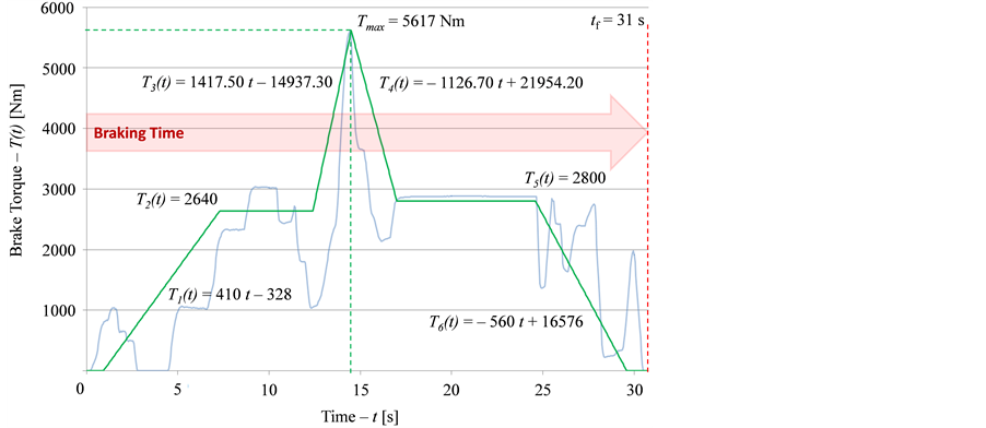
Figure A.1. Linear approach of brake torque variation.
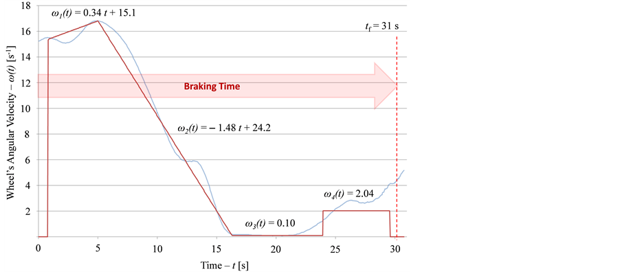
Figure A.2. Linear approach of wheel’s angular velocity.
Table A.1. Maximum contact pressure and maximum friction force per unit of area, function of time.
Table A.2. Calculated data.
Table A.3. Maximum heat flux per unit of area, function of time.