Engineering
Vol. 3 No. 4 (2011) , Article ID: 4604 , 4 pages DOI:10.4236/eng.2011.34048
Stress Function of a Rotating Variable-Thickness Annular Disk Using Exact and Numerical Methods
1Department of Mathematics, Faculty of Science, King AbdulAziz University, Jeddah, Saudi Arabia
2Department of Mathematics, Faculty of Science, Kafrelsheikh University, Kafr El-Sheikh, Egypt
E-mail: zenkour@gmail.com
Received January 31, 2011; revised March 18, 2011; accepted March 31, 2011
Keywords: Rotating, Annular Disk, Variable Thickness, Runge-Kutta Method
ABSTRACT
In this paper, the exact analytical and numerical solutions for rotating variable-thickness annular disk are presented. The inner and outer edges of the rotating variable-thickness annular disk are considered to have free boundary conditions. Two different annular disks for the radially varying thickness are given. The numerical Runge-Kutta solution as well as the exact analytical solution is available for the first disk while the exact analytical solution is not available for the second annular disk. Both exact and numerical results for stress function, stresses, strains and radial displacement will be investigated for the first annular disk of variable thickness. The accuracy of the present numerical solution is discussed and its ability of use for the second rotating variable-thickness annular disk is investigated. Finally, the distributions of stress function, displacement, strains, and stresses will be presented. The appropriate comparisons and discussions are made at the same angular velocity.
1. Introduction
The annular disks have received a great deal of attention because of their widely used in many mechanical and electronic devices, such as computer disk memory units, circular saws, and turbine rotors. The problems of rotating annular disks can be easily found in most of the standard elasticity books [1,2]. Most of the research works are concentrated on the analytical solutions of rotating disks with simple cross-section geometries of uniform thickness and especially variable thickness [3-8]. In [6], the rotating annular disks are analytically studied and closed form solutions for the rotating disks subjected to various boundary conditions are obtained. In [7], the rotating viscoelastic solid and annular disks of exponentially varying thickness are studied by analytical means. The problem of an annular disk subjected to purely radial temperature variation is treated in [8]. The analytical solution for the analysis of thermal deformations and stresses in elastic annular disks with arbitrary cross-sections of continuously variable thickness is presented.
As many rotating components in use have complex cross-sectional geometries, they cannot be dealt with using the existing analytical methods. Numerical methods, such as the finite element method [9], the boundary element method [10] and Runge-Kutta’s algorithm [11-14], can be applied to cope with these rotating components. Both finite element method and Runge-Kutta's algorithm are used in [14]. Some additional numerical methods are used in the literature. In [15], the rotating annular disks with uniform and variable thicknesses and densities are solved using homotopy perturbation method and Adomian’s decomposition method.
This work is a predictive assessment of the stresses in and deformation of a rotating annular disk with variable thickness variation. Two methods of analysis, namely, the analytical method and Runge-Kutta numerical method of governing differential equations were used. This study concentrated first on the analytical solution for the rotating annular disk with arbitrary cross-section of continuously variable thickness. A unified governing equation will be first derived from the basic equations of the rotating disks and the proposed stress-strain relationship. Next, Runge-Kutta method is introduced to solve the governing equation. A comparison between both analytical and numerical solutions is made. The accuracy of the numerical solution is used to find the stress function, stresses, strains and displacement of rotating variable-thickness annular disk whose analytical solution is not available. Finally, a number of numerical examples are given to demonstrate the validity of the proposed method.
2. Basic Equations
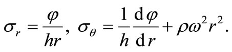
As the effect of thickness variation of rotating annular disks can be taken into account in their equation of motion, the theory of the variable-thickness annular disks can give good results as that of the uniform-thickness annular disks as long as they meet the assumption of plane stress. After considering this effect, the equation of motion of rotating disks with variable thickness can be written as
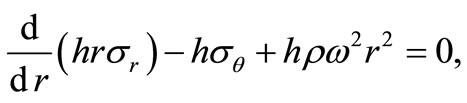 (1)
(1)
where  and
and  are the radial and circumferential stresses, r is the radial coordinate,
  is the density of the rotating disk,
  is the constant angular velocity, and h is the thickness which is function of the radial coordinate r.
The relations between the radial displacement u and the strains are irrespective of the thickness of the rotating disk. They can be written as
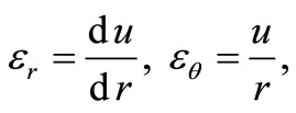 (2)
(2)
where  and
and  are the radial and circumferential strains, respectively. The above geometric relations lead to the following condition of deformation harmony:
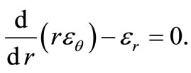 (3)
(3)
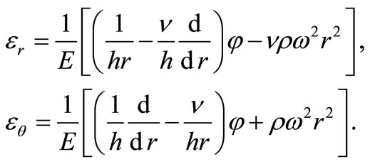
For the elastic deformation, the constitutive equations for the rotating disk can be described with Hooke’s law
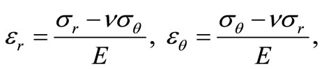 (4)
(4)
where E is Young’s modulus and  is Poisson’s ratio. Introducing the stress function
  and assuming that the following relations hold between the stresses and the stress function
 (5)
(5)
Substituting Equation (5) into Equation (4), one obtains
 (6)
(6)
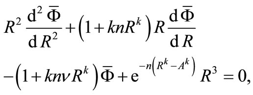
The substitution of Equation (6) into Equation (3) produces the following confluent hypergeometric differential equation for the stress function 
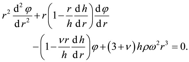 (7)
(7)
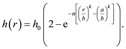
The thickness of the annular disk is assumed to vary nonlinearly through the radial direction. It is assumed to be in terms of a simple exponential power law distribution according to the following two types:
Disk 1:
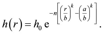 (8)
(8)
Disk 2:
 (9)
(9)
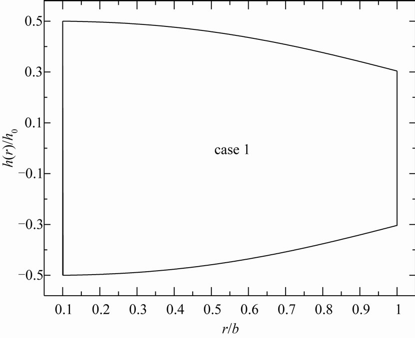
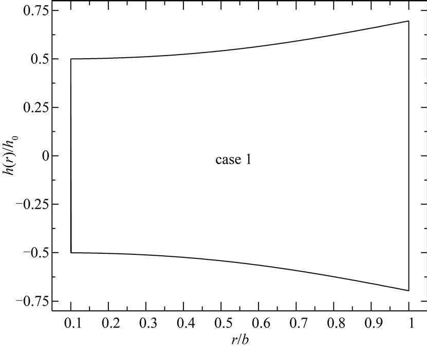
For both disks,  is the thickness at the inner edge of the disk, n and k are geometric parameters, a is the inner radius of the disk and b is the outer radius of the disk (see Figures 1 and 2). The value of n equal to zero represents a uniform-thickness annular disk. It is to be noted that the parameter n determines the thickness at the outer edge of the annular disk relative to
  while the parameter k determine the shape of the profile. The thickness of the annular disk 1 may be decreases at the outer edge (see Figure 1) while the thickness of the annular disk 2 may be increases at the outer edge (see Figure 2). The value of k equal to unity represents a linearly decreasing variable thickness for the annular disk 1 while it represents a linearly increasing variable thickness for the annular disk 2. The geometric parameters k and n are given according to three cases. In case 1: k = 2.5, n = 2, in case 2: k = 2.5, n = 0.5, and in case 3: k = 0.6, n = 2.
For small k and large n (case 3) the profile of the annular disk 1 is concave while it is convex for large k and small n (case 2). For large k and n (case 1) the profile of the annular disk 1 may be changing its shape from convexity to concavity. In addition, the profile of the annular disk 2 is convex for small k and large n (case 3) while it is concave for large k and small n (case 2). Also, for large k and n (case 3) the profile of the annular disk 2 may change its shape from concavity to convexity.
 (a)
(a)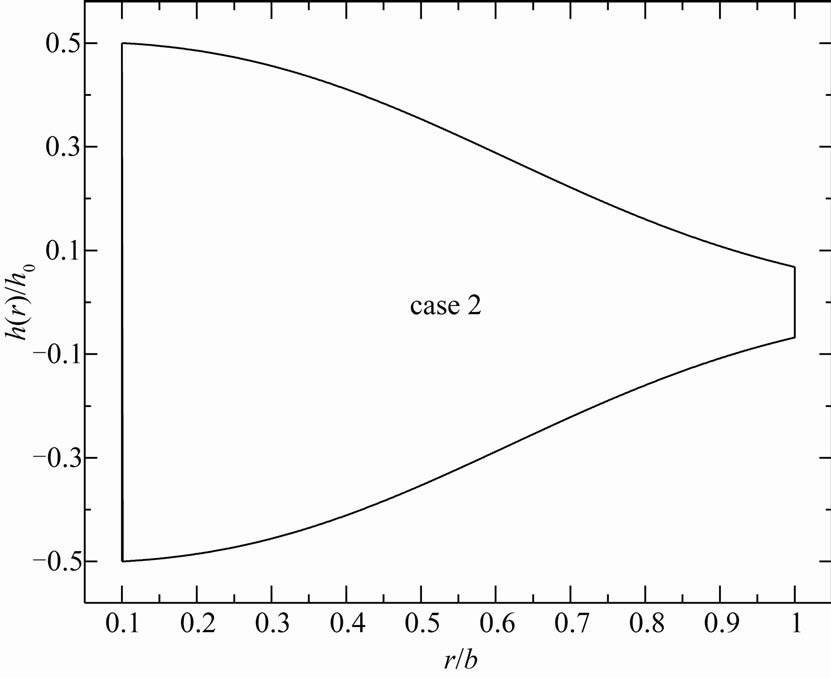 (b)
(b)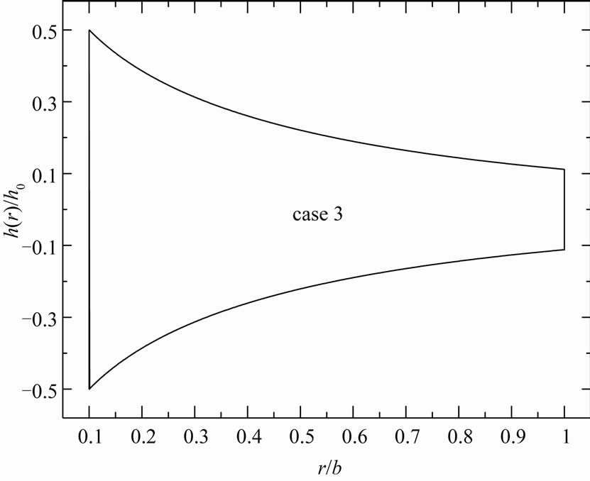 (c)
(c)
Figure 1. Variable-thickness annular disk 1 profiles for (a) case 1, (b) case 2 and (c) case 3.
 (a)
(a)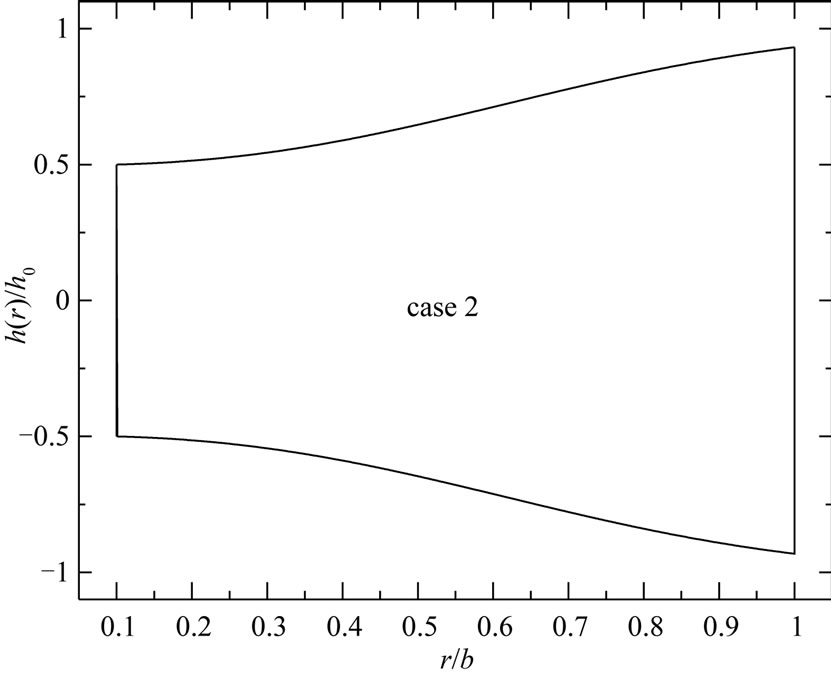 (b)
(b)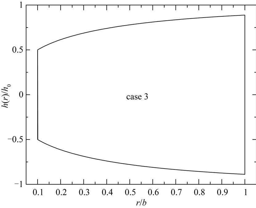 (c)
(c)
Figure 2. Variable-thickness annular disk 2 profiles for (a) case 1, (b) case 2 and (c) case 3.
To simplify the solving process, we introduce the following dimensionless variables:
 (10)
(10)
Then, Equation (7) may be written in the following simple forms according to the two cases:
 (11)
(11)
for annular disk 1, and
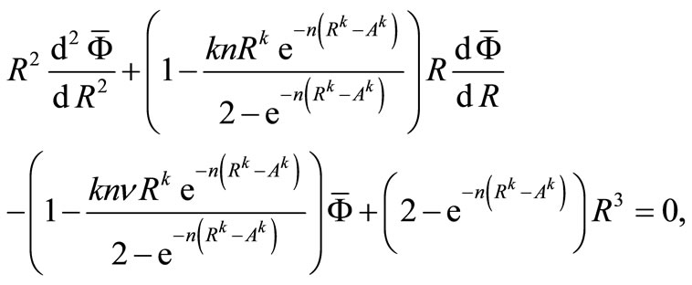 (12)
(12)
for annular disk 2.
3. Exact and Numerical Solutions
The exact general solution for Equation (11) may be available while it is not available for Equation (12). The modified Runge-Kutta numerical solution may be available for both cases. Firstly, we will get both the exact and numerical solutions for Equation (11). If the numerical solution is compared well with the exact one, we can use it to solve Equation (12) for the second case.
3.1. Exact Solution
The exact general solution for Equation (11) can be written as
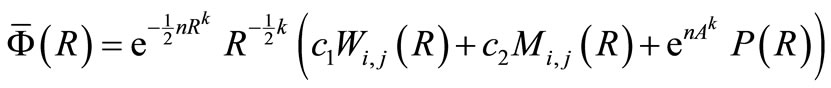 ,(13)
,(13)
where  and
and  are arbitrary constants and
 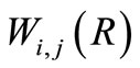 and
and  are Whittaker’s functions (see Abramowitz and Stegun [16]),
 (14)
(14)
in which
 (15)
(15)
It is to be noted that Whittaker’s functions may be given by
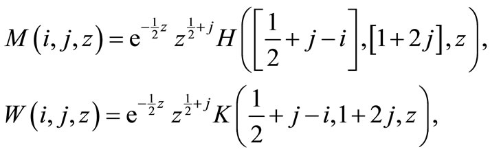 (16)
(16)
where H and K are the hypergeometric and Kummer’s functions, respectively, with n > 0. It is to be noted that for real values of i and j, Whittaker’s functions  and
and  converge for
 .
.
The term in Equation (13) can be written as
 (17)
(17)
where
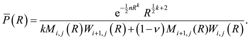 (18)
(18)
The substitution of Equation (13) into Equation (5) with the aid of the dimensionless forms given in Equation (10) gives the radial and circumferential stresses in the following forms:
 (19)
(19)
Note that the first differentiations of Whittaker’s functions  and
and  are given by
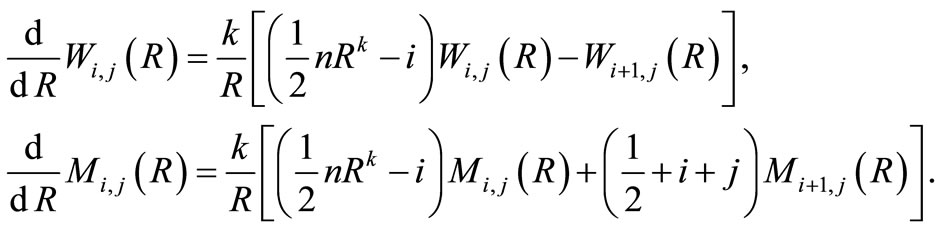 (20)
(20)
Finally, the dimensionless strains and the corresponding radial displacement may be obtained easily using Equation (19) as well as the dimensionless forms given in Equation (10). So, all of stress function, stresses, strains, and radial displacement can be completely determined under the traction conditions on the inner and outer surfaces of the annular disk. They can be expressed as
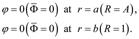 (21)
(21)
3.2. Numerical Solution
The modified Runge-Kutta algorithm may be used here to solve both the differential Equations (11) and (12) with the aid of the boundary conditions given in Equation (21). Equations (11) or (12) can be written in the following general form:
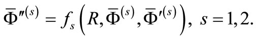 (22)
(22)
where the prime denotes differentiation with respect to R and s denotes the disk number. The functions  may be given by
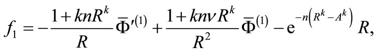 (23)
(23)
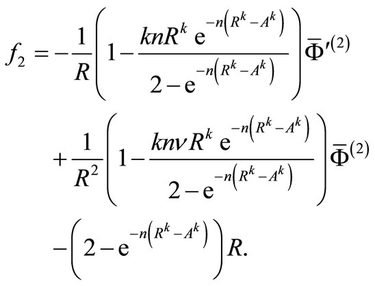 (24)
(24)
Runge-Kutta’s iterative formulae for the second-order differential equation are [11-14]
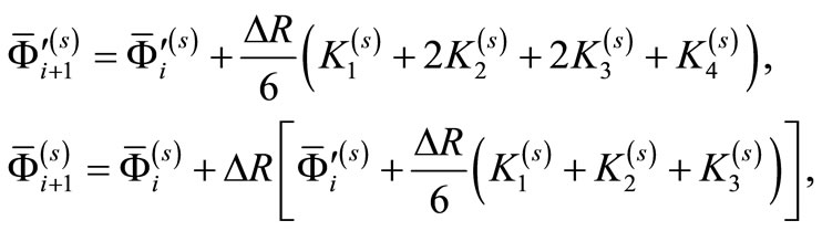 (25)
(25)
where  is the increment of the distance along the radial direction of the rotating annular disks, and
  can be determined with the following relations
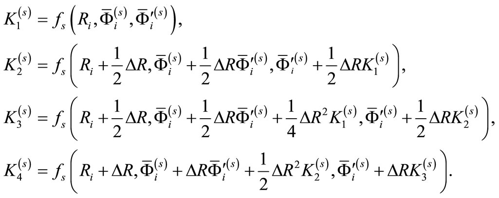 (26)
(26)
The numerical simulation starts from the inner boundary, where a trial value of the first derivative of the stress function is assumed. With a small distance , the stress function and its first derivative at the new position can be obtained using Equation (25) and the radial stress is calculated. According to the difference between the computed radial stress and the known radial stress at the outer boundary, the initial trial value of the first derivative of the stress function at the inner boundary is modified and the next iteration is carried out in the same way. This iterative process is performed until both the boundary conditions are simultaneously satisfied. Once the stress function is obtained, the stresses, strains, and displacement in the rotating annular disks can be obtained using Equations (2), (5) and (6) with the aid of the dimensionless given in Equation (10). This process may be easily done after getting the continuous form of the stress function using the curve fitting and least square method. So, all other quantities can be easily determined.
4. Numerical Examples and Discussion
Some numerical examples for the rotating variablethickness annular disk will be given according the exact and numerical solutions . Results determined as per the exact analytical solution are compared with those obtained by the numerical Runge-Kutta (R-K) solution in Figures 3-10 for disk 1. Additional results for stress function, radial displacement, strains and stresses of the rotating variable-thickness annular disk 2 using the numerical R-K solution are also presented in Figures 11-16. The inner and outer radii of the disk are taken to be a = 0.1 b (R = A = 0.1) and b (R = 1), and the results are given in terms of the rotating angular velocity.
The numerical applications will be carried out for the radial displacement, strains, stress function and stresses
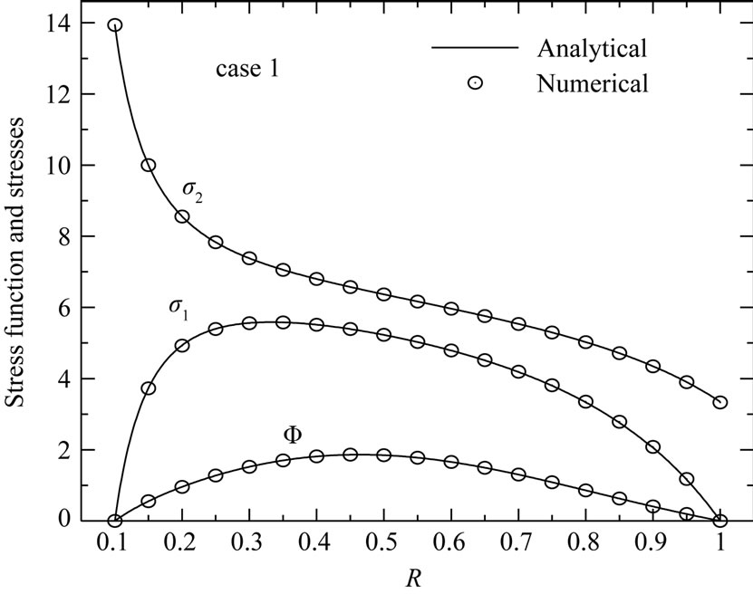
Figure 3. Stress function Ф, radial stress σ1 and circumferential stress σ2 in the variable-thickness annular disk 1.
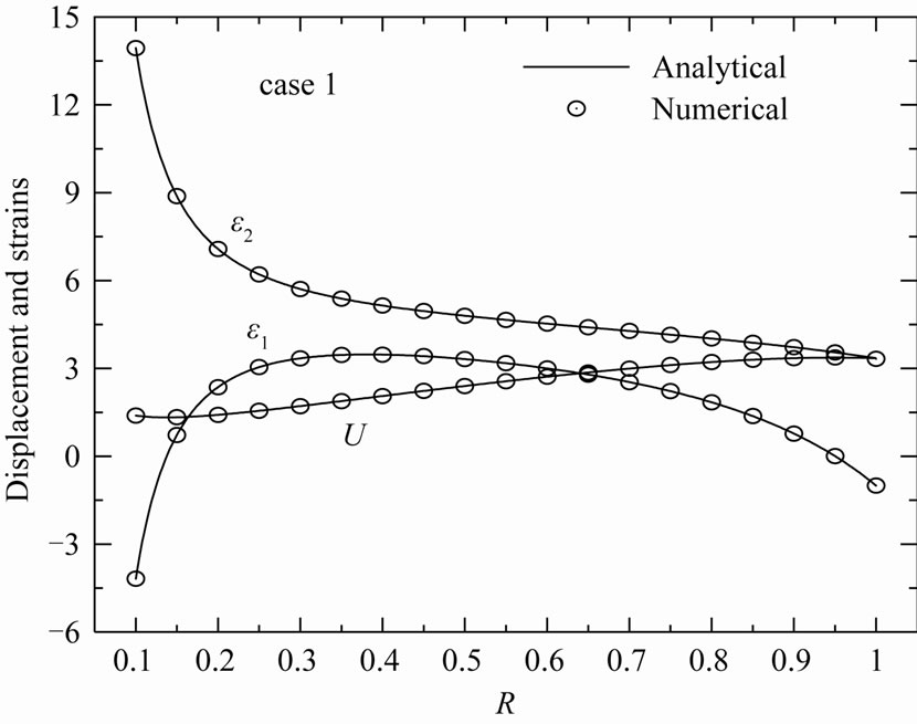
Figure 4. Displacement U, radial strain ε1 and circumferential strain ε2 in the variable-thickness annular disk 1.
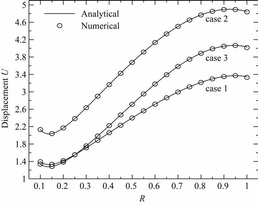
Figure 5. Displacement U of the variable-thickness annular disk 1 for all cases.
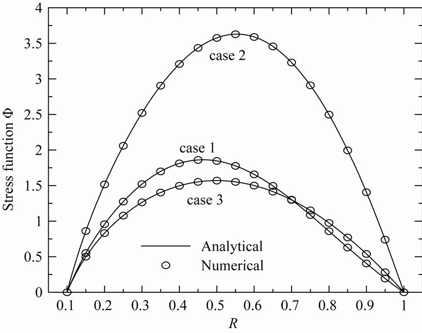
Figure 6. Stress function Ф of the variable-thickness annular disk 1 for all cases.
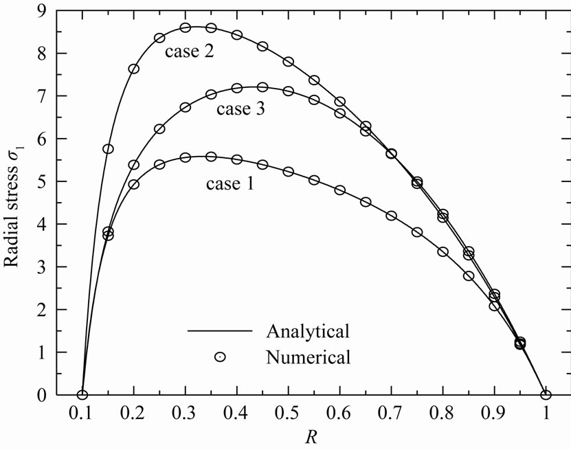
Figure 7. Radial stress σ1 in the variable-thickness annular disk 1 for all cases.
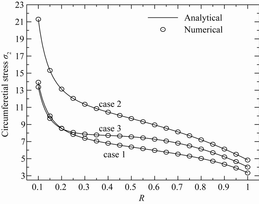
Figure 8. Circumferential stress σ2 in the variable-thickness annular disk 1 for all cases.
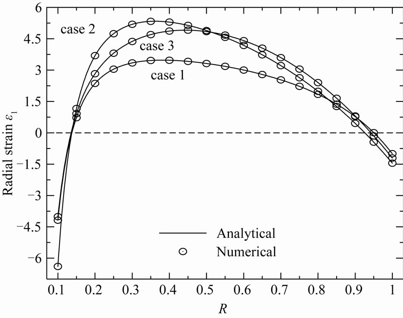
Figure 9. Radial strain ε1 in the variable-thickness annular disk 1 for all cases.
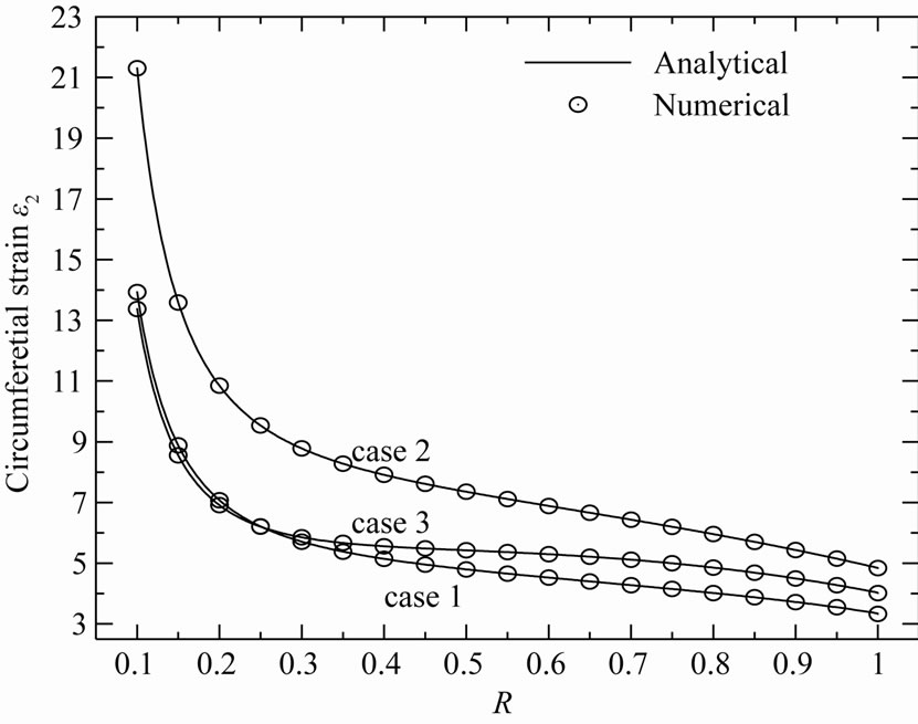
Figure 10. Circumferential strain ε2 in the variable-thickness annular disk 1 for all cases.
that being reported herein, with help of Equation (10), are in the following dimensionless forms:
 (27)
(27)
The distribution of the stress function and stresses are presented in Figure 3 while the distribution of the radial displacement and strains are presented in Figure 4. The results are given for rotating variable-thickness annular disk with k = 2.5 and n = 2 (case 1). The numerical R-K solution is compared with the exact analytical solution. It is clear that, R-K method gives all results with excellent accuracy when compared with the exact analytical solution.
The distributions of the stress functions, radial stress, circumferential stress, radial displacement, radial strain as well as circumferential strain through the radial direction of the annular disk 1 are all presented in Figures 5-10, respectively, for different cases of the geometric parameters k and n. Figure 5 shows that the radial displacement U has minimum value near the inner edge (at R = 0.15) and maximum value near the outer edge (at R = 0.9) for all cases of the parameters k and n. Cases 1 and 3 (n = 2) are coincided with each other when R = 0.2. Case 2 with small n (n = 0.5) gives the highest values of the displacement.
Figure 6 shows that the stress function  has its maximum at the mid-plane of the disk (R = 0.55) for case 2 while its maximum occurs at (R = 0.45) and (R = 0.5) for cases 1 and 3, respectively. Once again, cases 1 and 3 are coincided with each other when R = 0.7. Case 2 with small n gives the highest values of the stress function.
The radial stress  and circumferential stress
  in the rotating variable-thickness annular disk 1 are plotted in Figures 7 and 8. The maximum value of
  does not occur at the mid-plane of the disk 1. It occurs at R = 0.33, R = 0.43, R = 0.35 for cases 2, 3 and 1, respectively. The maximum value of
  occurs at the inner surface of the disk 1 while the smallest value occurs at outer surface. Case 1 gives the smallest stresses. The same conclusion may be applied on the plots of strains in Figures 9 and 10.
It can be seen from Figures 3-10 that the R-K method can describe all results through-the-thickness of the rotating annular disk 1 very well enough. This puts into evidence the great role played by R-K method in the modeling of rotating variable-thickness annular disks. So, it will trustily used to find the solution for Equation (12) of the rotating variable-thickness annular disk 2. As a result, the stresses and stress function in the rotating variable-thickness disk 2 are plotted in Figures 11-13 according to all cases. However, the radial displacement and strains are plotted in Figures 14-16.
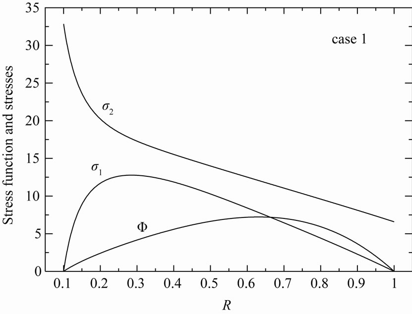
Figure 11. Stress function Ф, radial stress σ1 and circumferential stress σ2 in the variable-thickness annular disk 2 for case 1.
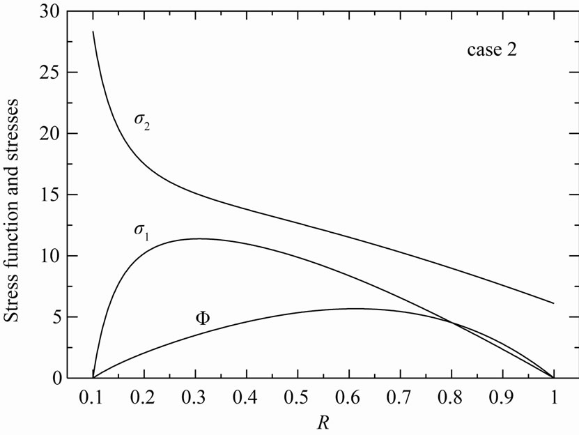
Figure 12. Stress function Ф, radial stress σ1 and circumferential stress σ2 in the variable-thickness annular disk 2 for case 2.
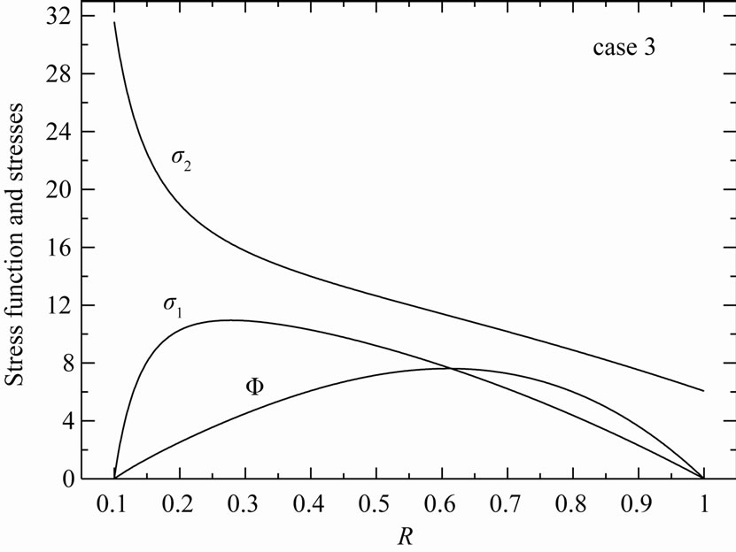
Figure 13. Stress function Ф, radial stress σ1 and circumferential stress σ2 in the variable-thickness annular disk 2 for case 3.
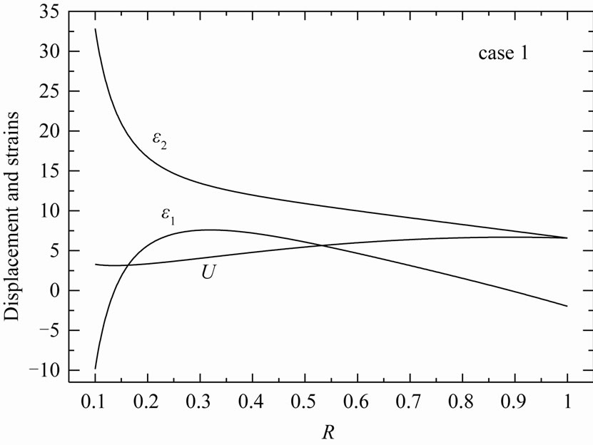
Figure 14. Displacement U, radial strain ε1 and circumferential strain ε2 in the variable-thickness annular disk 2 for case 1.
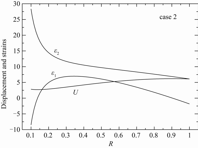
Figure 15. Displacement U, radial strain ε1 and circumferential strain ε2 in the variable-thickness annular disk 2 for case 2.
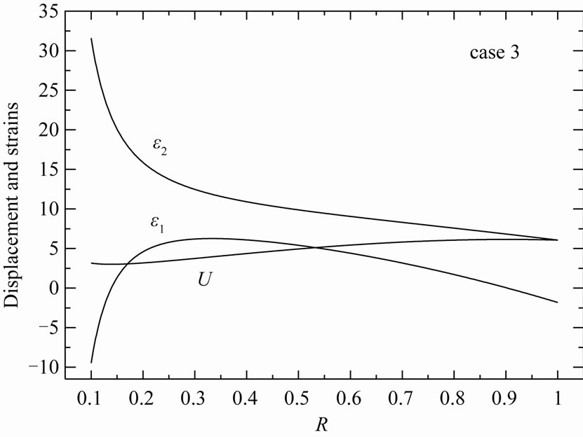
Figure 16. Displacement U, radial strain ε1 and circumferential strain ε2 in the variable-thickness annular disk 2 for case 3.
5. Conclusions
This paper presents an exact analytical solution for a rotating variable-thickness annular disk. Also, it presents a unified numerical method based on Runge-Kutta forth-order method for the elastic calculation of different rotating annular disks with a general, arbitrary configuration. The governing equation was derived from the equilibrium equation and the stress-strain relationship. The calculation of the rotating annular disk was turned into finding the solution of second-order differential equations under the given conditions at two boundary fixed points. Runge-Kutta method algorithm was introduced to solve the governing equation for two types of annular disks, in which the exact solution of one of them only is available. A number of numerical examples were studied. The results from the exact analytical and R-K solutions were compared. The proposed R-K approach gives very agreeable results to the exact analytical solution. The modified R-K method presented here may be trustily used for the boundary value problems that their exact solutions are not available.
6. REFERENCES
- S. P. Timoshenko and J. N. Goodier, “Theory of Elasticity”, McGraw-Hill, New York, 1970.
- S. C. Ugral and S.K. Fenster, “Advanced Strength and Applied Elasticity”, Elsevier, New York, 1987.
- U. Güven, “Elastic-Plastic Stresses in a Rotating Annular Disk of Variable Thickness and Variable Density,” International Journal of Mechanical Sciences, Vol. 34, 1992, pp. 133-138.
- U. Güven, “On the Stress in the Elastic-Plastic Annular Disk of Variable Thickness under External Pressure,” International Journal of Solids and Structures, Vol. 30, 1993, pp. 651-658.
- U. Güven, “Stress Distribution in a Linear Hardening Annular Disk of Variable Thickness Subjected to External Pressure,” International Journal of Mechanical Sciences, Vol. 40, 1998, pp. 589-601. doi:10.1016/S0020-7403(97)00081-7
- A. M. Zenkour, “Analytical Solutions for Rotating Exponentially-Graded Annular Disks with Various Boundary Conditions,” International Journal of Structural Stability and Dynamics, Vol. 5, 2005, pp. 557-577. doi:10.1142/S0219455405001726
- A. M. Zenkour and M. N. M. Allam, “On the Rotating Fiber-Reinforced Viscoelastic Composite Solid and Annular Disks of Variable Thickness,” International Journal for Computational Methods in Engineering Science & Mechanics, Vol. 7, 2006, pp. 21-31. doi:10.1080/155022891009639
- A. M. Zenkour, “Thermoelastic Solutions for Annular Disks with Arbitrary Variable Thickness,” Structural Engineering and Mechanics, Vol. 24, 2006, pp. 515-528.
- O. C. Zienkiewicz, “The Finite Element Method in Engineering Science,” McGraw-Hill, London, 1971.
- P. K. Banerjee and R. Butterfield, “Boundary Element Methods in Engineering Science,” McGraw-Hill, New York, 1981.
- M. L. James, G. M. Smith and J. C. Wolford, “Applied Numerical Methods for Digital Computation,” Harper & Row, New York, 1985
- L. H. You, Y. Y. Tang, J. J. Zhang and C.Y. Zheng, “Numerical Analysis of Elastic-Plastic Rotating Disks with Arbitrary Variable Thickness and Density,” International Journal of Solids and Structures, Vol. 37, 2000, pp. 7809-7820. doi:10.1016/S0020-7683(99)00308-X
- C. F. Gerald and P. O. Wheatley, “Applied Numerical Analysis,” 6th Edition, Addison-Wesley, California, 2002.
- M. H. Hojjati and A. Hassani, “Theoretical and Numerical Analysis of Rotating Discs of Non-Uniform Thickness and Density,” International Journal of Pressure Vessels and Piping, Vol. 85, 2008, pp. 694-700. doi:10.1016/j.ijpvp.2008.02.010
- M. H. Hojjati and S. Jafari, “Semi-Exact Solution of Elastic Non-Uniform Thickness and Density Rotating Disks by Homotopy Perturbation and Adomian’s Decomposition Methods. Part I: Elastic Solution,” International Journal of Pressure Vessels and Piping, Vol. 85, 2008, pp. 871-878. doi:10.1016/j.ijpvp.2008.06.001
- M. Abramowitz and I. Stegun, “Handbook of Mathematical Functions,” 5th Printing, US Government Printing Office, Washington, DC, 1966.