Journal of Modern Physics
Vol.09 No.02(2018), Article ID:81933,15 pages
10.4236/jmp.2018.92020
Infrared Polarizabilities of 3d-Transition and Rare-Earth Metals
Kofi Nuroh
Department of Mathematical Sciences, Kent State University, Salem, OH, USA

Copyright © 2018 by author and Scientific Research Publishing Inc.
This work is licensed under the Creative Commons Attribution International License (CC BY 4.0).
http://creativecommons.org/licenses/by/4.0/


Received: December 31, 2017; Accepted: January 21, 2018; Published: January 24, 2018
ABSTRACT
A transition or rare-earth metal is modeled as the atom immersed in a jellium at intermediate electron gas densities specified by . The ground states of the spherical jellium atom are constructed based on the Hohenberg-Kohn- Sham density-functional formalism with the inclusion of electron-electron self-interaction corrections of Perdew and Zunger. Static and dynamic polarizabilities of the jellium atom are deduced using time-dependent linear response theory in a local density approximation as formulated by Stott and Zaremba. The calculation is extended to include the intervening elements In, Xe, Cs, and Ba. The calculation demonstrates how the Lindhard dielectric function can be modified to apply to non-simple metals treated in the jellium model.
Keywords:
Infrared, Polarizability, Jellium, Transition Metals, Rare-Earth Metals, Electron Self-Interaction Correction

1. Introduction
The dynamical polarizability, and its corresponding static value, for metals, have been investigated theoretically by mainly using aggregate of particles to mimic the metal. In particular, has been shown to have an anomalous enhancement over its classical expected value of , where R is some characteristic radius of the metallic particle. In 1965, Gor’kov and Eliashberg (GE) [1] introduced the idea of exploring the electronic excitations of small metallic particles based on phenomenological temperature-dependent statistical mechanics. With this concept they provided an explanation to the anomalous enhancement in . This insight generated interest in the physics of small metallic particles and similar investigations ensued thereafter that exploited other theoretical methods. In general, these theoretical approaches may be classified into three grouping: those based on GEs original concept [2] - [15] , those that rely on random phase approximation (RPA) and its variants [16] [17] , and those that use self-consistent density-functional ideas [18] - [23] .
We utilize the following model as a means of mimicking the medal. A transition or a rare-earth metal atom is immersed in a uniform electron gas of density prescribed by , namely, the jellium model. The ground state of the spherical jellium atom consisting of the discrete core levels and the continuum valence states are determined using the density functional prescription of Perdew and Zunger [24] . Since the prescription includes correction for electron self-interactions, it would provide a more accurate account of electron-electron interactions. A Thomas-Fermi pseudopotential has been used as the external potential to determine the initial density of the system. This serves as input to the Hohenberg- Kohn-Sham density-functional scheme [25] [26] to be described in Section II. Once the self-consistent complete set of energies and wavefunctions
, (with and ) are determined, they are subjected to
a time-dependent linear density approximation (TDLDA) methods [27] [28] [29] [30] , that have been so successfully used to determine the polarizability of systems possessing spherical symmetry. The spherical jellium model is a crude one; nonetheless, calculations based on this model would serve as a first approximation for more realistic calculations that should have to incorporate the translational symmetry of the solid, especially in the transition metal atoms where the itinerant character of the valence states are crucial for many metallic properties.
In the jellium model, the response of the interacting electron gas to an external potential leads to a complex dynamic dielectric function . If the external potential is weak, linear response theory may be invoked leading to a complex polarization function . Further, if the lowest term contribution to , namely, is retained, then we get , where is proportional to .
The Lindhard expression for this quantity is given in, e.g., Fetter and Walecka [31] as
where the dimensionless energy parameter and momentum parameter are respectively given by and . If atomic units ( ) are used, then the input frequency is in rydbergs. Since is proportional to the absorption probability for transferring the four-momentum to the electron gas, we expect this quantity to be proportional to for some fixed . In the above, is the non-interacting complex frequency-dependent polarizability, and is its interacting counterpart. These quantities are the subjects of our investigation in this work to be outlined in Section IIA. In Figure 1, calculations for , for different momentum transfers are displayed. Figure 2 shows calculations of for some selected metals with . The semblance of the profiles in the two-panel- figure display suggests that using the spherical jellium model to represent the metal is a feasible one for the determination of the polarizability of metals.
2. Methods
1) The stationary state
We briefly review the Perdew-Zunger [24] theory of self-interaction correction (SIC) to density-functional approximations for many-body electron systems on which the calculations are based. According to this exposé, a stationary state of an atom or ion immersed in a uniform electron gas (the jellium) may be described, within the local-spin-density (LSD) approximation, by a charge density
(1)
where
(2)
is the density of an orbital with quantum numbers and , and or is the electronic spin, and fractional occupation numbers are

Figure 1. Real part of the Lindhard function. Upper graph panels: Dash plot ( ); Dash Dot plot ( ); Dash Dot-Dot plot ( ); Short Dash plot ( ); Solid line (sum of the q’s). Lower graph panel: Dash plot ( ); Dot plot ( ); Dash Dot plot ( ); Solid line (sum of the q’s).

Figure 2. Real part of . Dash plot (independent particle); Solid line (with interactions).
allowed . In this approximation, the set of one-electron orbitals satisfies a Schrödinger-like equation (in atomic units, )
(3)
The orbital-dependent potential is
(4)
In the above is the chemical potential [= −electronegativity] and is an external magnetic field that couples to the electron spin .
The self-interaction correction to the potential is the second curly bracket in Equation (4). The direct Coulomb potential is the expression
(5)
while the LSD exchange-correlation potential is
(6)
and is given by the functional derivative . The expression is the exchange-correlation energy per particle of an electron gas with the spin density . This makes it possible for the homogeneous system to be folded into calculations for the inhomogeneous systems like atoms and ions. For the detailed construct of the expressions in this section, the interested reader is referred to the original formulation in Reference [24] .
An iterative procedure is used to solve Equations (1)-(4). First, an initial guess is made for the spin and the spin orbital densities instead of using Equations ((1) and (2)). Then Equations ((3) and (4)) are solved using a direct predictor-corrector numerical integration. Thereafter, Equations (1)-(4) are successively solved until self-consistency is achieved with a relative accuracy of 10−6 in both sets of densities, or a relative accuracy of 10−6 in energy, whichever occurs first. The orbital densities are first sphericalized before evaluating the potential and the total energy. (A bar over any variable in an expression or equation signifies that the self-consistent value is used in evaluating it.) After a self-consistent set of orbitals is obtained, the total energy within the LSD may be computed as
(7)
Again, the more prescribed calculational details are left for the interested reader to consult with the original paper of Reference [24] .
2) Linear response and polarizability
In Section IIA the stationary states are set up to perform spin-polarized calculation. From now onward, we drop the bars on quantities in Section IIA. We set so that the calculation is now spin non-polarized. Further, we drop the spin label and take the set of quantum labels . According to the theory of linear response, if an arbitrary system of electrons is perturbed by an external potential it induces a deviation in its density from its ground state value given by
(8)
The quantity is the frequency-dependent response function for the interacting electron system. On the other hand, if the density fluctuation is viewed as arising from an induced effective potential for the system, then it may equivalently be represented as
(9)
Here is the non-interacting response function for the fermion system, and the effective potential is given by
(10)
with
, (11)
where it is considered that . A popular approximation to the exchange-correlation energy is the local density approximation (LDA) in which is simply taken as a function of the density, and Equation (11) becomes
(12)
The response function is an embodiment of all possible excitations from the ground state to excited states . The eigenfunctions and eigenenergies will be presumed to be solutions to the Kohn-Sham equations
(13)
(14)
(15)
where is the electrostatic Hartree potential and is the exchange- correlation potential.
Following the approach of Reference [28] , the non-interacting response function may be expressed in terms of retarded Green’s function as
(16)
where the summation is over the occupied states and
(17)
Rather than using Equation (17) to determine the non-interacting susceptibility in Equation (16), the retarded Green’s function can be directly obtained as the solution to the differential equation of Equation (13),
, (18)
with the appropriate outgoing wave boundary conditions.
3) Response function with spherical symmetry
Since we are dealing with a spherical jellium atom, it becomes convenient to work in spherical harmonics and write
(19)
and
. (20)
The application of a uniform frequency-dependent electric field to the spherical atom corresponds to an external potential
(21)
If Equations ((20) and (21)) are substituted into Equation (16), only the dipolar component couples to the external perturbation Equation (21) and the non-interacting dipolar response function is
(22)
where
. (23)
From Equation (17) the harmonic component representation of the retarded Green’s function becomes
, (24)
and we have written . But as has been remarked earlier, the daunting task of performing the summation over single-particle radial orbitals can be circumvented since from Equation (18), is a solution to the inhomogeneous radial differential equation
, (25)
which satisfies the appropriate boundary conditions at the origin and at infinity. Following earlier observations [28] , if E corresponds to a bound state energy then can be expressed in terms of solutions to the radial homogeneous equation at energy :
. (26)
The harmonic component Green’s function is then given by
. (27)
Here is the solution of Equation (26) that behaves asymptotically for as and is the solution which is regular at the origin; W refers to the Wronskian of the two solutions. If E does not correspond to a bound state energy, Equation (27) is further simplified by normalizing such that it behaves asymptotically as . In this case becomes
, (28)
where and .
For the spherical jellium atom, the induced density can be expressed as
. (29)
Putting this result in Equation (9) using Equation (10) leads to a linear integral equation for the position-dependent polarizability as
, (30)
where
, (31)
On the other hand, the application of the perturbation of Equation (21) gives rise to the induced dipole moment
(32)
in the spherical atom. Using Equation (29) we infer from Equation (32) that
. (33)
But the dynamic polarizability is related to the induced dipole moment and the applied field as
. (34)
Substituting this value of into Equation (33) yields the complex frequency-dependent polarizability as
. (35)
3. Results and Discussion
The prescription contained in Section IIC has been used to calculate , the imaginary part of the polarizability, for the transition metals (TMs) and for the rare earth metals (REMs), including calculations for some intervening metals. The results of these calculations using Equation (35) are displayed for the TMs (Figure 3 and Figure 4), for the intervening metals In, Cs, Xe, and Ba (Figure 5), and for the REMs (Figures 6-8). The breaks in the graphs are those energy input ranges for which there were convergence problems in the numerical procedure. The dashed curves represent the independent particle or non-interacting polarizabilities in which the Coulomb and exchange-correlation interactions are switched off. The solid curves have those interactions present.
The static polarizabilities have been calculated for the jellium atoms of the transition metals and the rare earth metals. These are compared with the density functional-based code for the neutral atoms of these systems by Zangwill and Liberman [32] , and the results are displayed in Figure 9. In the case of the TMs both the neutral and jellium atoms show monotonically decreasing static polarizabilities with increasing atomic number (Z). In fact, the values may be fitted to an exponential decay function of the form
, (36)
with the following values for the parameters , , and with an adjusted for the neutral atoms, while the values

Figure 3. Imaginary part of for Sc, Ti, V, Cr, Mn, Fe: Dash plot (independent particle); Solid line (with interactions).

Figure 4. Imaginary part of for Co, Cu, Ni, Zn: Dash plot (independent particle); Solid line (with interactions).

Figure 5. Imaginary part of for In, Xe, Cs, Ba: Dash plot (independent particle); Solid line (with interactions).

Figure 6. Imaginary part of for La, Ce, Pr, Nd: Dash plot (independent particle); Solid line (with interactions).

Figure 7. Imaginary part of for Pm, Sm, Eu, Gd, Tb, Dy: Dash plot (independent particle); Solid line (with interactions).

Figure 8. Imaginary part of for Ho, Er, Tm, Yb: Dash plot (independent particle); Solid line (with interactions).
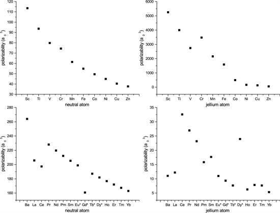
Figure 9. Static polarizabilities for the TMs and REMs for the jellium and neutral atoms.
for the jellium atoms are , , and with an adjusted . The function defined in Equation (36) should not be construed as portraying dynamics of the atomic systems. Its purpose is to see trends in the atomic numbers with respect to the static polarizabilities.
In the case of the REMs there were instabilities in the numerical procedure yielding spurious negative values for the polarizabilities for some of the systems when the 4f states were included. Hence, they were frozen. These are the systems with asterisk marks in Figure 9. For the neutral atoms, if we exclude the obvious outliers , then the rest of the systems may be fitted to an exponential decay function like the one of Equation (36). The values of the fitted parameters are , , and , with an adjusted R-square value of 0.99865. Likewise for the jellium atoms if the outliers , and 66 are excluded, the rest of the systems may be fitted to Equation (36) with the parameters , , and with an adjusted .
4. Conclusions
The calculations portray extensive enhancement in the real part of the polarizabilities of the jellium atom is compared to the Lindhard counterpart, in support of the observations made by Gor’kov and Eliashberg in their pioneer work based on aggregate of particles to mimic metals, and subsequently validated by others.
Except for few elements, both the jellium TM and REM static polarizabilities show monotonically decreasing values with increasing atomic number just as the corresponding neutral atomic counterparts. Because of the localized nature of the 4f-states in REMs, often the neutral atomic values of polarizabilities are taken to represent the metallic without recourse to incorporating the band structure of the solid state. Magnitude-wise, the calculations presented here suggest that they would be different from the metallic counterparts if band-structure calculations exploiting the translational symmetry of the solid state are included. In that case, the values reported here for the REMs (as well as the TMs) would be a good gauge for such calculations.
Acknowledgements
The author is indebted to professors Zaremba and Stott for making available the jellium atom code and would also like to thank the referee for pointing out some minor but invaluable corrections.
Cite this paper
Nuroh, K. (2018) Infrared Polarizabilities of 3d-Transition and Rare-Earth Metals. Journal of Modern Physics, 9, 287-301. https://doi.org/10.4236/jmp.2018.92020
References
- 1. Gor’kov, L.P. and Eliashberg, G.M. (1965) Soviet Physics JETP, 21, 940-947.
- 2. Strässler, S., Rice, M.J. and Wider, P. (1972) Physical Review B, 6, 2575-2577. https://doi.org/10.1103/PhysRevB.6.2575
- 3. Lushnikov, A.A and Simonov, A.J. (1973) Physics Letters A, 44, 45-46. https://doi.org/10.1016/0375-9601(73)90953-5
- 4. Rice, M.J., Scheider, W.R. and Strasser, S. (1973) Physical Review B, 8, 474-482. https://doi.org/10.1103/PhysRevB.8.474
- 5. Schmidt-Ott, A., Schurtenberger, P. and Siegmann, H.C. (1980) Physical Review Letters, 45, 1284-1287. https://doi.org/10.1103/PhysRevLett.45.1284
- 6. Dasgupta, B.B. and Fuchs, R. (1981) Physical Review B, 24, 554-561. https://doi.org/10.1103/PhysRevB.24.554
- 7. Penn, D.R. and Rendell, R.W. (1981) Physical Review Letters, 47, 1067-1070. https://doi.org/10.1103/PhysRevLett.47.1067
- 8. Burtscher, H. and Schmidt-Ott, A. (1982) Physical Review Letters, 50, 1734-1737. https://doi.org/10.1103/PhysRevLett.48.1734
- 9. Thoai, D.B.T and Ekardt, W. (1982) Solid State Communications, 41, 687-690. https://doi.org/10.1016/0038-1098(82)90732-3
- 10. Wood, D.H. and Ashcroft, N.W. (1982) Physical Review B, 25, 6255-6274. https://doi.org/10.1103/PhysRevB.25.6255
- 11. Ekardt, W., Thoai, D.B.T., Frank, F. and Schulze, W. (1983) Solid State Communications, 46, 571-574. https://doi.org/10.1016/0038-1098(83)90694-4
- 12. Apell, P. (1984) Physica Scripta, 29, 146-149. https://doi.org/10.1088/0031-8949/29/2/010
- 13. Kreibig, U. and Genzel, L. (1985) Surface Science, 156, 678-700. https://doi.org/10.1016/0039-6028(85)90239-0
- 14. Persson, B.N.J. (1993) Surface Science, 281, 153-162. https://doi.org/10.1016/0039-6028(93)90865-H
- 15. Blanter, Y.M. and Mirlin, A.D. (1996) Physical Review B, 53, 12601-12604. https://doi.org/10.1103/PhysRevB.53.12601
- 16. Lushnikov, A.A. and Simonov, A.J. (1974) Zieitschrift für Physik, 270, 17-24. https://doi.org/10.1007/BF01676788
- 17. Zaremba, E. and Persson, B.N.J. (1987) Physical Review B, 35, 596-606. https://doi.org/10.1103/PhysRevB.35.596
- 18. Snider, R. and Sorbello, R.S. (1983) Physical Review B, 28, 5702-5710. https://doi.org/10.1103/PhysRevB.28.5702
- 19. Ekardt, W. (1984) Physical Review B, 29, 1558-1564. https://doi.org/10.1103/PhysRevB.29.1558
- 20. Ekardt, W. (1984) Physical Review Letters, 52, 1925-1928. https://doi.org/10.1103/PhysRevLett.52.1925
- 21. Beck, D.E. (1984) Physical Review B, 30, 6935-6942. https://doi.org/10.1103/PhysRevB.30.6935
- 22. Ekardt, W. (1985) Physical Review B, 31, 6360-6370. https://doi.org/10.1103/PhysRevB.31.6360
- 23. Puska, M.J., Nieminen, R.M. and Manninen, A. (1985) Physical Review B, 31, 3486-3495. https://doi.org/10.1103/PhysRevB.31.3486
- 24. Perdew, J.P. and Zunger, A. (1981) Physical Review B, 23, 5048-5079. https://doi.org/10.1103/PhysRevB.23.5048
- 25. Hohenberg, P. and Kohn, W. (1964) Physical Review B, 136, 864-871. https://doi.org/10.1103/PhysRev.136.B864
- 26. Kohn, W. and Sham, L.J. (1965) Physical Review A, 140, 1133-1138. https://doi.org/10.1103/PhysRev.140.A1133
- 27. Zangwill, A. and Soven, P. (1980) Physical Review A, 21, 1561-1572. https://doi.org/10.1103/PhysRevA.21.1561
- 28. Stott, M.J. and Zaremba, E. (1980) Physical Review A, 21, 12-23. https://doi.org/10.1103/PhysRevA.21.12
- 29. Nuroh, K., Stott, M.J. and Zaremba, E. (1982) Physical Review Letters, 49, 862-866. https://doi.org/10.1103/PhysRevLett.49.862
- 30. Nuroh, K., Zaremba, E. and Stott, M.J. (1987) Giant Resonances in the 4d Subshell Photoabsorption Spectra of Ba, Ba+, and Ba++. In: Connerade, J.P., Esteva, J.M. and Karnatak, R.C., Eds., Giant Resonances in Atoms, Molecules, and Solids, Plenum Press, New York, 115-135. https://doi.org/10.1007/978-1-4899-2004-1_6
- 31. Fetter, A.L. and Walecka, J.D. (1971) Quantum Theory of Many-Particle Systems. McGraw-Hill, New York.
- 32. Zangwill, A. and Liberman, D.A. (1984) Computer Physics Communications, 32, 63-73. https://doi.org/10.1016/0010-4655(84)90008-0