Journal of Modern Physics
Vol.07 No.10(2016), Article ID:67539,15 pages
10.4236/jmp.2016.710106
Dynamics of Nerve Pulse Propagation in a Weakly Dissipative Myelinated Axon
Nkeh Oma Nfor1, Mebu Tatason Mokoli2
1Complex Systems and Theoretical Biology Group, Laboratory of Research on Advanced Materials and Nonlinear Science(LaRAMaNS), Department of Physics, Faculty of Science, University of Buea, Buea, Cameroon
2Laboratory of Research on Advanced Materials and Nonlinear Science (LaRAMaNS), Department of Physics, Faculty of Science, University of Buea, Buea, Cameroon

Copyright © 2016 by authors and Scientific Research Publishing Inc.
This work is licensed under the Creative Commons Attribution International License (CC BY).
http://creativecommons.org/licenses/by/4.0/


Received 3 May 2016; accepted 17 June 2016; published 21 June 2016
ABSTRACT
We analytically derived the complex Ginzburg-Landau equation from the Liénard form of the discrete FitzHugh Nagumo model by employing the multiple scale expansions in the semidiscrete approximation. The complex Ginzburg-Landau equation now governs the dynamics of a pulse propagation along a myelinated nerve fiber where the wave dispersion relation is used to explain the famous phenomena of propagation failure and saltatory conduction. Stability analysis of the pulse soliton solution that mimics the action potential fulfills the Benjamin-Feir criteria for plane wave solutions. Finally, results from our numerical simulations show that as the dissipation along the myelinated axon increases, the nerve impulse broadens and finally degenerates to front solutions.
Keywords:
Ginzburg-Landau Equation, Liénard Form, Fitz Hugh Nagumo Model, Semidiscrete Approximation, Saltatory Conduction, Benjamin-Feir Criteria, Dissipation

1. Introduction
Wave propagation and pattern formation in a variety of excitable media can be effectively described by reaction-diffusion equations. The FitzHugh Nagumo (FHN) model [1] [2] is one of the simple examples of a two-dimensional excitable dynamics that governs such systems. This model have been used as a simplified version of the Hodgkin-Huxley model [3] of neuron firing. The FHN model which is characterized by a recovery mechanism furnishes us with a better understanding of the essential dynamics of the interaction of membrane potential and qualitatively captures the general properties of an excitable membrane. Even though its simplicity allows very valuable insight to be gained, the accuracy of reproducing real experimental results is limited.
Myelinated axons modelled by discrete FHN equations incorporate a richer dynamics than its continuous counterparts. Also, the mathematical study of spatially discrete models is challenging because of special and poorly understood phenomena occurring in them that are absent if the continuum limit of these models is taken. For example, in the discrete FHN model, there exists a coupling threshold for its propagation while the con- tinuous system sustains propagation of all coupling strengths [4] - [7] . Enormous efforts to understand pro- pagation failure in FHN system were made by Booth et al. [6] , in which they considered slow recovery and very special limiting values of the parameters characterizing the bistable source and the spatial diffusivity in the FHN system. By imposing some special boundary conditions, they studied the evolution of localized front from one cell to another until it failed to propagate. Also, by using the Morris-Lecar model for myelinated nerve fiber, Hastings et al. [8] demonstrated that travelling waves could be observed even though they had difficulties to extend their results to the FHN system. Our main focus is to capture the various profiles of nerve impulses along a myelinated axon when the dissipative effects is reduced to its minimum value. This will be experimentally very difficult to be realized, but we hope to theoretically investigate this effect by using perturbation techniques.
The effects of dissipation is prominent in most physical and biological systems [9] - [11] , such as the myelinated FHN fiber which is a discrete system made of periodic structures called Ranvier nodes [12] . Dissipative systems are spatiotemporally organized patterns that are far from a steady state configuration because of the dynamic imbalance between spatial interactions and temporal instabilities. This dissipative effect spread thoughout a neural network because of the spatially localized connectivity between adjacent group of neurons, leading to the diffusive transmissions to neighboring cells. In fact, from experimental and theoretical standpoint, waves travelling over dissipative neural network mostly vanish due to collision [13] - [15] and lack of an external energy source to take care of attenuation [16] . However, we still observe localized short excitations of nerve impulses [17] , ultrashort pulses from passively mode-locked lasers, travelling waves in cortical networks, Bose-Einstein condensates in cold atoms [18] , in various autonomous dissipative media, suggesting that more stable solitonic profiles can be observed provided measures are taken to minimize dissipation.
The control of pulse propagation in dissipative media can also be achieved by subjecting the system to high frequency periodic perturbations. For a discrete system like myelinated axons, this method has the advantage that the external frequency can either suppress or enhance the pulse propagation [19] . The purpose of this study is to examine the evolution of a nerve impulse, responsible for carrying electrical signals along a weakly dissipative myelinated axon. This issue is brought into sharp focus because neurons effectively participate in a collective spatiotemporal sharing of vital information. For some conservative media like in optical fibers, such crucial signals are conveyed by trains of solitons [20] - [22] which are robust to external perturbations. We derived the Complex Ginzburg-Landau (CGL) equation from a weakly dissipative FHN model, where the pulse solution clearly depicts the action potential typical in neural networks. The linear stability analysis of the action potential generally shows that the nerve impulse is relatively unstable to small pertubations.
The rest of the work is organized as follows; in Section 2, after a brief introduction of the FHN model, we derived the model CGL equation in a weak dissipative medium using the multiple scale expansion in the semi-discrete approach. The analytic solution of the CGL equation is obtained in Section 3 following the method highlighted in [23] , to obtain the Pereira and Stenflo [24] pulse soliton solution. A linear stability analysis is carried out in Section 4 to check the robustness of the nerve impulse when subjected to a minimal perturbation. Consequently, the Benjamin-Feir criteria is satisfied from the qualitative analysis of the modulational instability. Numerical simulations of the CGL equation depict the evolution of the pulse soliton whose width increases as the dissipation increases. In the absence of dissipation, we observe a stable profile of the nerve impulse. Finally Section 5 gives a summary of the entire work.
2. Model Equations
We consider a one-dimensional chain of FitzHugh-Nagumo equations [1] [2] :
 (1a)
(1a)
 (1b)
(1b)
Here  and
and  are the membrane potential and the recovery variable respectively at the
  excitable membrane site known as Ranvier node. The recovery variable
  depicts the slow dynamics because the parameters
  For Equation (1a), the first term,
  , accounts for the positive feedback, where depo- larization enhances more depolarization through the voltage-gated sodium channel. The second term,
  , is a rapid negative feedback loop, corresponding to the auto-inactivation of the sodium channel. The third term
  represents a recovery process which may be physically responsible for regulating the outward potassium currents that oppose depolarization. The last term is the discrete diffusive term with coupling strength K, that is proportional to the difference in internodal currents through a given Ranvier node. The first term of (1b) i.e. a mainly measures the potassium leakage current while
  captures the activation of the voltage-gated po- tassium channel by the membrane potential
 , which increases the magnitude of
 . Lastly,
  controls the pumping of potassium ions out of the neuron.
Differentiating Equation (1a) with respect to time and substituting the value of  from (1b) yields
 (2)
(2)
where  and
and  are all constants.
System (2) is the Liénard form of the FHN model of a myelinated nerve fiber which may be considered as the modified form of the van der Pol equation. For , Equation (2) becomes the cubic Liénard equation with linear damping and it is sometimes regarded as a generalization of damped oscillations. Furthermore, within the linear regime and when the dissipation is neglected, we obtain the well known linear harmonic oscillator that finds numerous applications in both classical and quantum physics. The Liénard type of equations have been intensively investigated from both mathematical and physical perspectives, and their study remains an active field of research in mathematical physics [25] - [28] .
Equation (2) also mimics a one dimensional chain of atoms with unit mass, harmonically coupled to their nearest neighbors, characterized by dissipation and subjected to nonlinear on-site potential. A lot of difficulties is encountered to analytically solve this equation, however we will use a perturbation technique to minimize the effects of dissipation and also attempts to find appropriate solutions. In this light, all the dissipative coefficients  are perturbed to the order
 , where
  is a slow variable parameter. Also, we greatly minimize the rate at which the leakage potassium ions are discharged from the neuron by perturbing
  to order
 . Consequently keeping just terms up to order
 , Equation (2) is rewritten as
 (3)
(3)
There are always frequency limits within which normal propagation of nerve impulse signals are observed across the FHN myelinated axon. In order to define the appropriate frequency range, we employ a perturbative technique where a suitable solution of the FHN model containing  parameter is used. Upon substitution of this solution into the diffusive FHN model (3), the dispersion relation is obtained with terms at order of
 . Hence, we consider a simplified solution of our FHN model (3) of the form;
 (4)
(4)
with  where q is the normal mode wave number and
  is the angular frequency.
In the semidiscrete approximation,  is supposedly independent of the “fast” variables t and n. Instead, it depend on the “slow” variables defined by
  and
and , for
, for . A continuum limit approxi- mation is then made with the wave amplitudes while the discrete nature of the phase in maintained, details of this method is given in [25] [29] .
Collecting terms at order  gives the dispersion relation
 (5)
(5)
which is plotted in Figure 1. From Equation (5), the linear spectrum has a gap  and it is limited by
the cut-off frequency  due to discreteness.
The variation of the diffuseness of the plasma membrane through the dispersion coefficient , physically

Figure 1. Linear dispersion curve of the nerve impulse for  and
and . There is a lower cutoff mode
  with frequency
  and upper cutoff mode
  with frequency
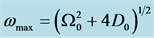 .
.
accounts for the alteration of ions movement across pumps and ion channels at the Ranvier nodes. Clearly for normal propagation of action potential across the myelinated axon, there exists a frequency range ,
,
where  (lower cutoff mode
 ) and
) and  (upper cutoff mode
 ). In
). In
this frequency range, the voltage-gated sodium ions channels are highly concentrated in the Ranvier nodes which are myelin free. When an action potential is generated at the axon hillock, the influx of sodium ions causes the adjacent Ranvier nodes to depolarize, resulting in an action potential at the node. This also triggers depolarization of the next Ranvier node and the eventual initiation of an action potential. Action potentials are successively generated at neighboring Ranvier nodes; therefore, the action potential in a myelinated axon appears to jump from one node to the next, a process called saltatory conduction. For , the action potential initially generated from one Ranvier node jumps to the next in a discontinuous manner. This process allows the speed of conduction to be greatly increased and completely distorts switching between adjacent Ranvier nodes. Consequently, this leads to propagation failure because of the inability of the nerve impulse to move across the axon. Lastly, for
 , the nerve impulse can not propagate because its amplitude exponentially decays to zero. However considering the nonlinearity of the medium, it may be possible to observe normal propagation along the axon provided the amplitude exceeds a certain threshold value. This mode of propagation called supratransmission has been realized in many physical systems [30] - [33] .
Terms of order  gives
gives
 (6)
(6)
where  is the group velocity as depicted in Figure 2.
Finally, we collect terms proportional to  to have
 (7)
(7)
By considering the reference mobile frame  and
and  with
with  being the group velocity of
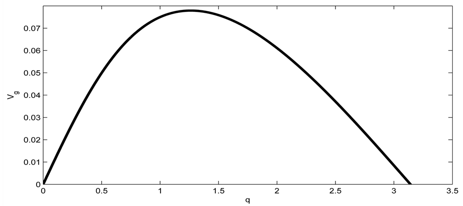
Figure 2. Group velocity of the nerve impulse for  and
and .
.
the wave, we obtain
 (8)
(8)
where P, is the real dispersion coefficient,  are respectively the real and imaginary parts of the nonlinear coefficient, while
  is the dissipative coefficient that causes the attenuation of action potential because of lost of energy during propagation. These parameters are given by;
 (9)
(9)
 (10)
(10)
 (11)
(11)
 (12)
(12)
Equation (8) is the CGL equation and generally speaking, it represents one of the most-studied nonlinear equations in the physics world today. This is because it gives a qualitative and quantitative description of a myriad of physical activities [11] [25] [34] . In neural networks, the propagation of modulated nerve impulses observed is governed by CGL equation, which clearly demonstrates how neurons participate in processing and sharing of information [25] . In this study which we focus on the propagation of action potential along a myelinated axon, it is incumbent on us to obtain appropriate solutions that depicts the asymmetric structural features of action potential. Physically in most conservative media [35] , solitary waves are understood as carriers of energy, however in this our context where dissipation is still prominent we need to balance the energy outflow in order to observe stable nerve impulses.
3. Solution of the Equation of Motion
Since we are dealing with a CGL equation, it is incumbent on us to look for a propagating wave solution of the form:
 (13)
(13)
which upon substitution into Equation (8) to obtain
 (14a)
(14a)
 (14b)
(14b)
Let us assume that
 (15)
(15)
where d is the chirp parameter and  is an arbitrary phase which we set to zero (i.e.
 ) without loss of generality. Equation (15) is obviously a constraint imposed on
  because the chirp could have a more general functional dependence on
 . However this restriction allows us to find all possible analytic pulse-like solutions of the modified CGL Equation (8). Consequently, Equation (14) becomes
 (16a)
(16a)
 (16b)
(16b)
We now have two second order ordinary differential equations (ODE) relative to the same dependent variable, . To have a common solution, the two equations must be compatible which generally in most systems is not the case. However, for this particular system, they can be made compatible by a proper choice of the parameters.
The following procedure is employed in order to find the compatibility conditions of the two equations; initially we eliminate the first derivatives from Equation (16) to have
 (17)
(17)
which upon integration and setting the integration constant to zero yields
 (18)
(18)
On the other hand, we eliminate the second derivative from Equation (16), obtaining
 (19)
(19)
Equations (18) and (19) must coincide, consequently leading to the following conditions:
 (20)
(20)
In order for us to obtain pulse solutions with real amplitudes, we assume that  and without loss of generality, we set
 , leading to
 . The solution of CGL Equation (8) obtained by by Pereira and Stenflo [24] now reads
 (21)
(21)
with the amplitude of the solution plotted in Figure 3.
We now obtain the exact analytic solution of the nerve impulse propagating along the myelinated axon by substituting (21) into the FHN model solution (4) to have;
 (22)
(22)
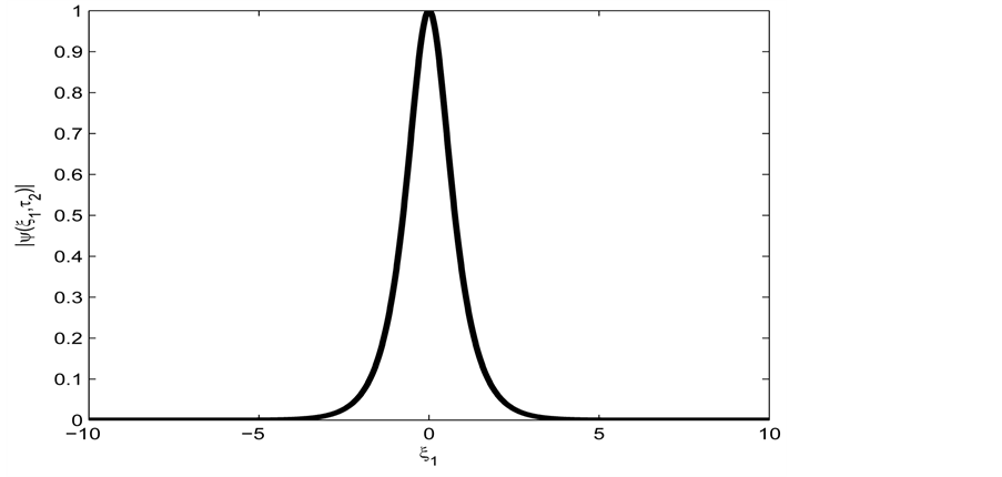
Figure 3. Spatial solution (21) of the CGL Equation (9), for 

 and
and .
.
where

Figure 4 depicts the spatial profile of this nerve impulse which may be considered as an electrical signal that propagates over a long distance without a change in amplitude.
Also, when the parameter  is varied, the form of the wave is greatly distorted as in Figure 5. Finally, Figure 6 depicts the spatiotemporal
4. Linear Stability and Numerical Analysis
Stability is a very important property of a wave profile in a neural network, since it determines whether such patterns can be observed experimentally, or utilized for diagnostic purposes. Recall that the phenomenon of modulational instability results when a steady-state solution is subjected to a weak perturbation, which eventually leads to the exponential growth of its amplitude along the line of propagation due to the interplay between the nonlinearity and dispersive effects of the medium. Initially, we consider the stability of the trivial homogeneous solution  by substituting the perturbations of the form
  in the linearized part of Equation (8). This leads to the characteristic equation
 (23)
(23)
where q is a spatial wavenumber of the perturbation and  determines the growth rate. The corresponding dispersion relation reads
 (24)
(24)
and when all the eigenvalues  have negative real parts, the homogeneous solution is asymptotically stable. Clearly the stability depends on the dissipative coefficient R and we conclude that the trivial solution is unstable since
 .
.
We now study the existence and stability of plane wave solutions  of Equation (8). We obtain the relation between the unknown amplitude
 , wavenumber q and frequency
  of the plane wave solution as follows;
 (25)
(25)

Figure 4. Spatial solution (22) of the FHN model (3), for 
 and
and .
.
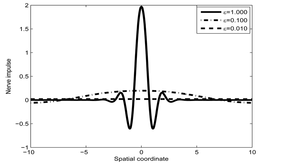
Figure 5. Spatial variation of solution (22) of the FHN model (3) as parameter  is varied. This is for
  and
and .
.
Due to the symmetry property of the CGL Equation (8) i.e.  this equation is symmetric under the reflection
 , and we restrict our analysis to the case
 . The real and imaginary parts of Equation (25) give the expressions for the amplitude
  and the frequency
  at a given wavenumber q:
 (a)
(a)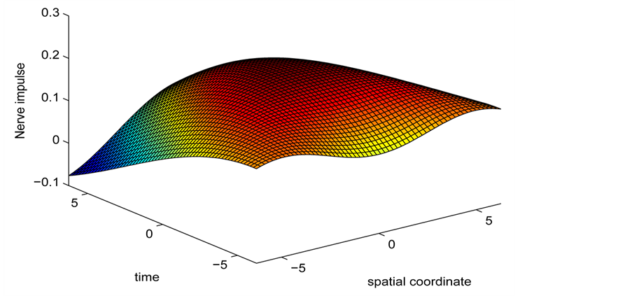 (b)
(b)
Figure 6. Spatiotemporal evolution of nerve impulse solution (22) for 
 . (a)
. (a)  (b)
(b) .
.
 (26)
(26)
Figure 7 shows the amplitude of the plane wave solution  as a function of the dissipative parameter
  (since
 ) for
) for .
.
We now perturb the plane wave solutions in order to have
 (27)
(27)
where
 (28)
(28)
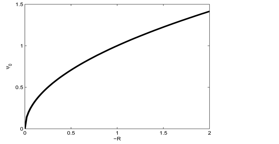
Figure 7. Amplitude of plane wave solution  versus parameter
  for
for  according to Equation. (26).
is a small perturbation term with a growth rate . Here
  and
and  denote complex conjugation, and k stands for different perturbation modes. Substitution of (27) into CGL Equation (8) and linearization in
  yields
 (29)
(29)
After substituting (28) into (29) and using Equation (25), we obtain an equation involving two linearly independent functions  and
and . Requiring that the coefficients of these functions are zero, we arrive at a system of linear equations for the unknowns
  and
and :
:
 (30)
(30)
with


Since we are looking for non-trivial solutions , the characteristic equation for the perturbation growth rate
  is obtained when the determinant of the coefficient matrix vanishes:
 (31)
(31)
Solutions  can now be found explicitly and the maximum of their real parts determines the stability of plane waves. Consequently we solve Equation (31) to obtain
 (32)
(32)
where  is the discriminant of the quadratic Equation (31). It is a very useful
component because it determines the nature of roots of the growth rate  which is purely complex. Since this discriminant depends on different perturbation modes k, it is therefore clear that
  is bound to have multiple values as will be demonstrated below.
For  plane waves are modulationally stable since
For  implying that
  we have that
  and the plane waves are
always stable since 
Lastly, for  implying that
  we have that
 . The perturbation
grows exponentially with time resulting to the instability of the plane waves which tend to self-modulate with a wave vector k. The plane wave solutions of the CGL Equation (8) clearly manifest the the classical Benjamin- Feir scenario where plane waves are unstable for positive , while they are stable for negative values. Consequently, one expects to find spatially localized nerve impulses along the myelinated axon, for any wave carrier whose wave vector is in the positive range of
 .
.
The condition , is also the condition for the existence of solitons, the study of the long-term evolution of a plane wave injected as initial condition in the neural network shows that, after a period during which the waves start to self-modulate as predicted by the linear stability analysis we just performed, this change persists until the amplitude of the plane waves vanishes in some regions. Sometimes, this modulational instability leads to a train of pulses [36] , but for our case, this effect generates a single nerve impulse produced by the superposition of continuous waves oscillating at a constant frequency shift.
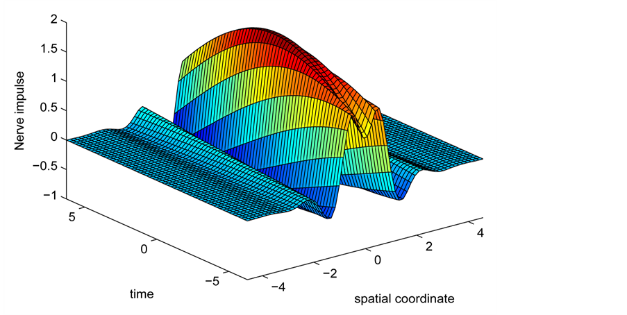
We now perform the numerical simulations of the CGL Equation (8) by using a Runge-Kutta scheme with fixed step size and initial conditions obtained from the analytic solution (21) of the CGL equation to check the long term effects of modulational instability. Figure 8 depicts the spatiotemporal evolution of the nerve impulse along the myelinated axon as the dissipative parameter is varied.
In the first case, i.e. Figure 8(a) where the dissipation is zero, we observe that the pulse conserves its shape, indicating that energy is not lost during propagation. This creates an ideal platform where vital information is transmitted along the myelinated axon with little or no distortion. As the dissipation increases as in Figure 8(b) & Figure 8(c), the nerve impulse becomes wider and flatter and may be termed a flat-top soliton. As time tends to infinity, the flat top solitons becomes unstable and decomposes into two fronts.
The corresponding contour plot of the spatiotemporal evolution of the nerve impulse in Figure 8 is given by Figure 9. This numerical results clearly confirms the prediction of our linear stability analysis by demonstrating that solutions for  are unstable, and furnishes us with the details beyond the linear limits. This shows that the nerve impulse degenerates to fronts which are also solutions of the CGL equation [37] .
5. Conclusions
In this study, we addressed the issue of nerve pulse propagation along a weakly dissipative myelinated axon modelled by the discrete FHN model. The effect of dissipation is always a big nuisance during the transmission of electrical signals across a neural network, consequently crucial information is always lost. We transformed the FHN model to its Liénard form and minimized the effects of dissipation by perturbing the appropriate parameters to higher order. The proposed solution for the Liénard equation carried the  parameter, where the dispersion relation that governed the propagation of nerve impulse was obtained at the first order of terms in
 . The second and third order terms in
  gave the group velocity and the CGL equation respectively. The pulse soliton solution of the CGL equation was derived analytically, and clearly mimiced the action potential typical in neural networks. We carried out liner stability analysis in Section 4, with results showing that the pulse soliton was generated as a result of modulational instability of the plane wave solution. By numerically integrating the CGL equation and varying the dissipation, we demonstrated that nerve impulses conserved its shape in a dissipative free medium. As the myelinated axon becomes more and more dissipative, the nerve impulse
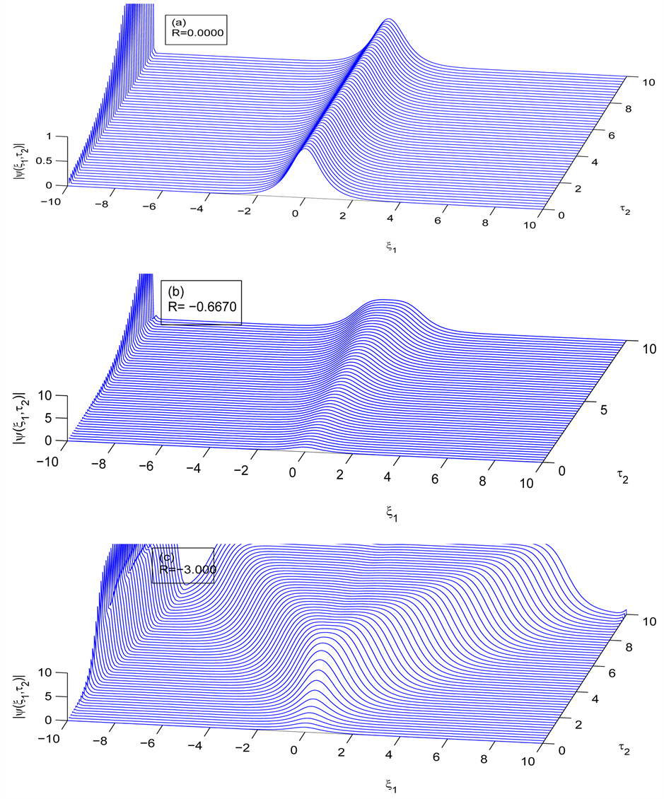
Figure 8. Spatiotemporal evolution of nerve impulse when the dissipation is varied for  (a)
(a) , (b)
, (b) , (c)
, (c)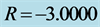 .
.
becomes more unstable and degenerates to fronts.
From this theoretical study carried on a dissipative myelinated axon, we believe it will furnish us with the appropriate knowledge of predicting the physiological state of real neurons. For instance, a sick neuron which is usually considered as dissipative can be clearly distinguished from a healthy neuron and consequently lead to
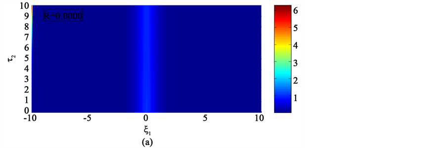
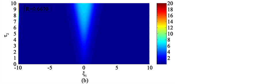
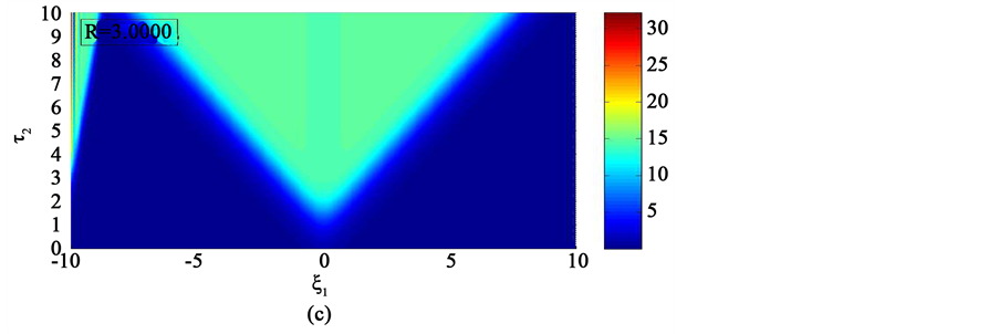
Figure 9. Corresponding contour plot of the evolution of bright nerve impulse in Figure 8 when the dissipation is varied for  (a)
(a) , (b)
, (b) , (c)
, (c) .
.
the appropriate therapeutic action.
Acknowledgements
N. Oma Nfor appreciates the enriching discussion with F. M. Moukam Kakmeni of the LaRAMaNS research group. The authors are very grateful to the referee for useful comments and the Journal of Modern Physics for subsidizing the publication fee.
Cite this paper
Nkeh Oma Nfor,Mebu Tatason Mokoli, (2016) Dynamics of Nerve Pulse Propagation in a Weakly Dissipative Myelinated Axon. Journal of Modern Physics,07,1166-1180. doi: 10.4236/jmp.2016.710106
References
- 1. FitzHugh, R.A. (1961) Biophysics Journal, 1, 445-446.
http://dx.doi.org/10.1016/S0006-3495(61)86902-6 - 2. Nagumo, J., Arimoto, S. andYoshitzawa, S. (1962) Proceedings of the IRE, 50, 2061-2070.
http://dx.doi.org/10.1109/JRPROC.1962.288235 - 3. Hodgkin, A.L. and Huxley, A.F. (1952) The Journal of Physiology, 117, 500-544.
http://dx.doi.org/10.1113/jphysiol.1952.sp004764 - 4. Keener, J.P. (1987) SIAM Journal on Applied Mathematics, 47, 556-572.
http://dx.doi.org/10.1137/0147038 - 5. Erneux, T. and Nicolis, G. (1993) Physica D: Nonlinear Phenomena, 67, 237-244.
http://dx.doi.org/10.1016/0167-2789(93)90208-I - 6. Booth, V. and Erneux, T. (1995) SIAM Journal on Applied Mathematics, 55, 1372-1389.
http://dx.doi.org/10.1137/S0036139994264944 - 7. Carpio, A. and Bonilla, L.L. (2001) Physical Review Letters, 86, 6034.
http://dx.doi.org/10.1103/PhysRevLett.86.6034 - 8. Hastings, S.P. and Chen, X. (1999) Journal of Mathematical Biology, 38, 1-20.
http://dx.doi.org/10.1007/s002859970001 - 9. Nicolis, G. andPrigogine, I. (1977) Self-Organization in Nonequilibrium Systems: From Dissipative Structures to Order through Fluctuations. Wiley, New York.
- 10. Haken, H. (1983) Synergetics: An Introduction. 3rd Edition, Springer, Berlin.
http://dx.doi.org/10.1007/978-3-642-88338-5 - 11. Kuramoto, Y. (1984) Chemical Oscillations, Waves, and Turbulence. Springer, Berlin.
http://dx.doi.org/10.1007/978-3-642-69689-3 - 12. Keener, J. and Sneyd, J. (2001) Mathematical Physiology. Springer, Berlin.
- 13. Wu, J.Y., Guan, L. and Tsau, Y. (1999) The Journal of Neuroscience, 19, 5005-5015.
- 14. Murray, J.D. (2002) Mathematical Biology II: Spatial Models and Biomedical Applications. 3rd Edition, Springer-Verlag, New York.
- 15. Lu, Y., Sato, Y. and Amari, S. (2011) Neural Computation, 23, 1248-1260.
http://dx.doi.org/10.1162/NECO_a_00111 - 16. Chang, W., Ankiewicz, A., Soto-Crespo, J.M. and Akhmediev, N. (2008) Physical Review A, 78, 023830.
http://dx.doi.org/10.1103/PhysRevA.78.023830 - 17. Dikande, A.M. and Bartholomew, G.A. (2009) Physical Review E, 80, 041904.
http://dx.doi.org/10.1103/PhysRevE.80.041904 - 18. Akhmediev, N. and Ankiewicz, A. (2008) Dissipative Solitons: From Optics to Biology and Medicine. Springer, Berlin.
- 19. Ratas, I. and Pyragas, K. (2012) Physical Review E, 86, 046211.
- 20. Fandio, D.J. J., Dikande, A.M. and Sunda-Meya, A. (2015) Physical Review A, 92, 053850.
http://dx.doi.org/10.1103/PhysRevA.92.053850 - 21. Amrani, F., Niang, A., Salhi, M., Komarov, A., Leblond, H. and Sanchez, F. (2011) Optics Letters, 36, 4239-4241.
http://dx.doi.org/10.1364/OL.36.004239 - 22. Haboucha, A., Leblond, H., Salhi, M., Komarov, A. and Sanchez, F. (2008) Physical Review A, 78, 043806.
- 23. Akhmediev, N.N. and Afanasjev, V.V. (1996) Physical Review E, 53, 1190-1201.
- 24. Pereira, N.R. and Stenflo, L. (1977) Physics of Fluids, 20, 1733-1734.
http://dx.doi.org/10.1063/1.861773 - 25. Kakmeni, F.M.M., Inack, E.M. and Yamakou, E.M. (2014) Physical Review E, 89, 052919.
http://dx.doi.org/10.1103/PhysRevE.89.052919 - 26. Pandey, S.N., Bindu, P.S., Senthilvelan, M. and Lakshmanan, M. (2009) Journal of Mathematical Physics, 50, 102701.
http://dx.doi.org/10.1063/1.3204075 - 27. Banerjee, D. and Bhattacharjee, J.K. (2010) Journal of Physics A: Mathematical and Theoretical, 43, 062001.
http://dx.doi.org/10.1088/1751-8113/43/6/062001 - 28. Messias, M. and Gouveia, M.R.A. (2011) Physica D: Nonlinear Phenomena, 240, 1402-1409.
http://dx.doi.org/10.1016/j.physd.2011.06.006 - 29. Dauxois, T. and Peyrard, M. (2006) Physics of Solitons. Cambridge University Press, Cambridge.
- 30. Khomeriki, R. (2004) Physical Review Letters, 92, 063905.
http://dx.doi.org/10.1103/PhysRevLett.92.063905 - 31. Susanto, H. (2008) SIAM Journal on Applied Mathematics, 69, 111-125.
http://dx.doi.org/10.1137/070698828 - 32. Susanto, H. and Karjanto, N. (2008) Journal of Nonlinear Optical Physics & Materials, 17, 159-165.
http://dx.doi.org/10.1142/S0218863508004147 - 33. Motcheyo, T.A.B., Tchawoua, C., Siewe, M.S. and Tchameu, J.D.T. (2013) Communications in Nonlinear Science and Numerical Simulation, 18, 946-952.
http://dx.doi.org/10.1016/j.cnsns.2012.09.005 - 34. Pismen, L.M. (1999) Vortices in Nonlinear Fields. Oxford University/Clarendon Press, Oxford/New York.
- 35. Newell, A.C. (1985) Solitons in Mathematics and Physics. SIAM, Philadelphia.
http://dx.doi.org/10.1137/1.9781611970227 - 36. Akhmedieva, N.N., Eleonski, V.M. and Kulagin, N.E. (1985) Soviet Physics—JETP, 62, 894-899.
- 37. Marcq, P., Chaté, H. and Conte, R. (1994) Physica D: Nonlinear Phenomena, 73, 305-317.
http://dx.doi.org/10.1016/0167-2789(94)90102-3