Received 22 August 2015; accepted 24 October 2015; published 28 October 2015

ABSTRACT

In this paper, I show that an interpretation of quantum mechanics using two-state vector formalism proposed by Aharonov, Bergmann, and Lebowitz, can solve one of the measurement problems formulated by Maudlin. According to this interpretation, we can simultaneously insist that the wave function of a system is complete, that the wave function is determined by the Schrödinger equation, and that the measurement of a physical quantity always has determinate outcomes, although Maudlin in his formulation of the measurement problem states that these three claims are mutually inconsistent. Further, I show that my interpretation does not contradict the uncertainty relation and the no-go theorem.

Keywords:

Two-State Vector Formalism, Measurement Problem, No-Go Theorem

1. Introduction

In his formalization of one of the measurement problems, Maudlin asserts that the following three claims are mutually inconsistent [1] :

A The wave function of a system is complete; i.e., the wave function specifies (directly or indirectly) all of the physical properties of a system.

B The wave function always evolves according to a linear dynamical equation (e.g., the Schrödinger equation).

C The measurement of, e.g., the spin of an electron, always (or at least usually) has determinate outcomes; i.e., at the end of the measurement, the measuring device is in a state that indicates either spin up (and not down) or spin down (and not up).

According to Maudlin, since these three claims are mutually inconsistent, all interpretations of quantum mechanics and alternative theories have to discard at least one of these claims. For example, hidden variable theories (e.g., Bohm mechanics and modal interpretations) deny statement A above, the so-called collapse theories deny statement B, and the many-worlds interpretation denies statement C. In this paper, I suggest an interpretation that consistently satisfies all the three abovementioned conditions. However, statement B is slightly modified as follows:

B' The wave function at a given time can always be determined according to a linear dynamical equation (e.g., the Schrödinger equation).

Statements A, B' and C are also mutually inconsistent in the existing interpretations. The new interpretation makes it possible to satisfy these three claims by considering not only the past state but also the future state of the given system. This interpretation is inspired by the two-state vector formalism (TSVF), which is a formalism of quantum mechanics proposed by Aharonov, Bergmann, and Lebowitz [2] .

TSVF has a rule, which is called the “ABL rule” and expressed in Equation (1) (“ABL” is an abbreviation of Aharonov, Bergmann, and Lebowitz), which determines the probability that the system under consideration is in a given state at t that is dependent on the states of the system at and . The ABL rule asserts that when the state of the system at is an eigenstate of a physical quantity Q, the probability that the state of the system at t is the eigenstate of Q is always 1. Further, we have to use the Schrödinger equation in order to calculate the probabilities by using the ABL rule. Therefore, there is no need to discard any of the above- mentioned three claims.

2. Brief Review of Two-State Vector Formalism

In this section, I present a brief review of TSVF. Let us assume that the physical quantity Q has eigenstates 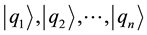(in this paper, we assume “the eigenstate-eigenvalue link”). The probability, , that the state of the system at t is is calculated as follows by using the ABL rule:

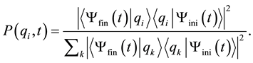(1)

Here,

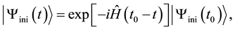(2)

where denotes the initial state of the system measured at and represents the final state of the system measured at, with. Equation (2) indicates that the wave functions in TSVF obey the Schrödinger equation.

There appears to be no method for verifying the prediction made using TSVF because we cannot know the intermediate state at t without destroying the state. Aharonov and Vaidman solved this problem by proposing a new measurement concept called “weak measurement”; measurements made according to this concept do not destroy the intermediate quantum state [3] .

According to Aharonov and Vaidman, the mean value obtained by weak measurement is the real part of the “weak value.” The weak value of the physical quantity Q at t, , is

(3)

Recently, physicists performed a weak measurement and confirmed that the theoretically predicted and measured weak values showed good agreement (cf. [4] ). Finally, with respect to the speculation that TSVF contradicts conventional quantum mechanics (CQM), it has been proved that the Born rule (and the ABL rule) can be derived in TSVF [5] .

3. How to Solve the Measurement Problem

In general, when the final state is an eigenstate, , of Q, the intermediate state is also with certainty because

(4)

Thus, we can simultaneously insist that the wave function of a system is complete, that the wave function is determined by using the Schrödinger equation (when the initial and final wave functions are given), and that the measurement of a physical quantity always (or at least usually) has determinate outcomes [6] .

Nevertheless, this interpretation still appears to be problematic in the following situation: Let us assume that we measure the x-spin of an electron at and obtain a value. Thus, the system state is, where and respectively represent the states in which the measured values of the x(z)-spin are and. Thereafter, we measure the z-spin of the electron at and obtain a value; thus, the system state is.

According to the ABL rule, both probabilities, namely, the probability that the system state at t is and the probability that the system state at t is, are 1. However, a quantum system cannot have the eigenstates of both the x-spin and the z-spin simultaneously. Let us assume that the state of a system is an eigenstate of non-commutative observables and having eigenvalues and, respectively. Consequently,. This contradicts the assumption that and are non-commutative.

Therefore, Aharonov, Popescu, and Tollaksen state that if at t we measure the spin in the z-direction, we must find it up, because that’s how the particle is prepared at. On the other hand, if at t we measure the spin along x, we must also find it up, because otherwise the measurement at wouldn’t find it up ([7] , p. 27).

Nonetheless, there is still concern that our interpretation contradicts the uncertainty relation (Kennard-Rober- tson inequality). Let us assume that an ensemble of electrons whose x-spin at is and z-spin at is has been prepared, and let us divide this ensemble into two sub-ensembles: and. When we perform a weak measurement of the x-spin in and the z-spin in at t, we obtain the result that the x-spin is and the z-spin is with certainty. This result indicates that the standard deviations of both the x-spin in and the z-spin in are 0 (because all the measurement results of the x-spin in and the z-spin in are). This result appears to contradict the uncertainty relation.

However, note that the uncertainty relation considers only the past state. When we consider the future state as well, the standard deviations of both the z-spin and the x-spin can be 0 at t. Here, we define

(5)

where denotes an operator of the z-spin. Consequently, we can easily obtain

(6)

Similarly, we can obtain. Therefore, when we interpret as the standard deviation of the z-spin in TSQM, it is not strange that the standard deviations of both the x-spin in and the z-spin in are 0.

In general, when we define

(7)

where Q denotes an observable quantity, represents an eigenstate of Q, and, we can easily obtain

(8)

when the final state is an eigenstate of Q.

Nevertheless, the concern that the abovementioned interpretation may contradict no-go theorem such as the Kochen-Specker theorem remains [8] . However, we can easily infer from Mermin’s version of the Kochen- Specker theorem [9] that there might not be any contradiction when only the x-spin and the -spin are determined because the Kochen-Specker theorem holds only when more than two axes of spin are determined.

Further, Tollaksen states that the weak value of spin changes according to the context of the experiment. For

example, he showed that there is a case where even though and , where represents the weak value of the j-spin of particle i (=1,2) [10] .

4. Conclusions

In this paper, I show that the following three claims can be simultaneously satisfied when we accept the interpretation of two-state vector formalism.

A The wave function of a system is complete; i.e., the wave function specifies (directly or indirectly) all of the physical properties of a system.

B' The wave function at a given time can always be determined according to a linear dynamical equation (e.g., the Schrödinger equation).

C The measurement of, e.g., the spin of an electron always (or at least usually) has determinate outcomes; i.e., at the end of the measurement, the measuring device is in a state that indicates either spin up (and not down) or spin down (and not up).

The key point is that when we measure a physical quantity Q and obtain a definite value q, the probability that the state of the system is the eigenstate of Q whose eigenvalue is q is 1.

Further, I show that this interpretation does not contradict the uncertainty relation and the Kochen-Specker theorem.

Acknowledgements

I thank the editor and the referee for their comments. This work was supported by JSPS KAKENHI Grant Number 26370021. This support is greatly appreciated.

Cite this paper

KunihisaMorita, (2015) Measurement Problem and Two-State Vector Formalism. Journal of Modern Physics,06,1864-1867. doi: 10.4236/jmp.2015.613191

References

- 1. Maudlin, T. (1995) Three Measurement Problems. Topoi, 14, 7-15.
http://dx.doi.org/10.1007/BF00763473 - 2. Aharonov, Y., Bergmann, P.G. and Lebowitz, J.L. (1964) Time Symmetry in the Quantum Process of Measurement. Physical Review B, 134, 1410-1416.
http://dx.doi.org/10.1103/PhysRev.134.B1410 - 3. haronov, Y. and Vaidman, L. (1990) Properties of a Quantum System during the Time Interval between Two Measurements. Physical Review A, 41, 11-20.
http://dx.doi.org/10.1103/PhysRevA.41.11 - 4. Yokota, K., Yamamoto, T., Koashi, M. and Imoto, N. (2009) Direct Observation of Hardy’s Paradox by Joint Weak Measurement with an Entangled Photon Pair. New Journal of Physics, 11, Article ID: 033011.
http://dx.doi.org/10.1088/1367-2630/11/3/033011 - 5. Hosoya, A. and Koga, M. (2011) Weak Values as Context Dependent Values of Observables and Born’s Rule. Journal of Physics A: Mathematical and Theoretical, 44, Article ID: 415303.
http://dx.doi.org/10.1088/1751-8113/44/41/415303 - 6. Morita, K. (2015) Einstein Dilemma and Two-State Vector Formalism. Journal of Quantum Information Science, 5, 41-46.
http://dx.doi.org/10.4236/jqis.2015.52006 - 7. Aharonov, Y., Popescu, S. and Tollaksen, J. (2010) A Time-Symmetric Formulation of Quantum Mechanics. Physics Today, 63, 27-32.
http://dx.doi.org/10.1063/1.3518209 - 8. Kochen, S.B. and Specker, E.P. (1967) The Problem of Hidden Variables in Quantum Mechanics. Journal of Mathematics and Mechanics, 17, 59-87.
http://dx.doi.org/10.1512/iumj.1968.17.17004 - 9. Mermin, N.D. (1993) Hidden Variables and the Two Theorems of John Bell. Reviews of Modern Physics, 65, 803-815.
http://dx.doi.org/10.1103/RevModPhys.65.803 - 10. Tollaksen, J. (2007) Pre- and Post-Selection, Weak Values and Contextuality. Journal of Physics A: Mathematical and Theoretical, 40, 9033-9066.
http://dx.doi.org/10.1088/1751-8113/40/30/025