Journal of Modern Physics
Vol.06 No.04(2015), Article ID:55113,10 pages
10.4236/jmp.2015.64051
Grand Canonical Approach to an Interacting Network
A. Nicolaidis1, K. Kosmidis2,3, V. Kiosses1
1Theoretical Physics Department, Aristotle University of Thessaloniki, Thessaloniki, Greece
2Computing & Communications Center, Aristotle University of Thessaloniki, Thessaloniki, Greece
3School of Engineering and Science, Jacobs University Bremen, Campus Ring 1, Bremen, Germany
Email: nicolaid@auth.gr, bkios@physics.auth.gr, kosmask@auth.gr
Copyright © 2015 by authors and Scientific Research Publishing Inc.
This work is licensed under the Creative Commons Attribution International License (CC BY).
http://creativecommons.org/licenses/by/4.0/


Received 19 July 2014; accepted 24 March 2015; published 27 March 2015
ABSTRACT
We consider a network composed of an arbitrary number of directed links. We employ a grand canonical partition function to study the statistical averages of the network in equilibrium. The Hamiltonian is composed of two parts: a “free” Hamiltonian H0 attributing a constant energy E to each link, and an interacting Hamiltonian Hint involving terms quadratic in the number of links. A Gaussian integration leads to a reformulated Hamiltonian, where now the number of links appears linearly. The reformulated Hamiltonian allows obtaining the exact behavior in limiting cases. At high temperatures the system reproduces the behavior of the free model, while at low temperatures the thermodynamic behavior is obtained by using a renormalized chemical potential, μeff = μ + l, where l is the strength of the interaction. We also resort to a mean field approximation, describing accurately the system over the entire range of all dynamical parameters. A detailed Monte-Carlo simulation verifies our theoretical expectations. We indicate that our model may serve as a prototype model to address a number of different systems.
Keywords:
Complex Networks, Statistical Mechanics, Monte Carlo Simulations, Grand Canonical Ensemble

1. Introduction
We are used to wondering first about particles or states and then about their interactions. We are first to ask about what it is and afterwards how it is. In most of our models in physics, or other branches of science, a system is considered as a collection of objects, with interactions among the objects introduced at a later stage. The examples are abundant (Ising model, lattice QCD, etc). It is not unjustified to consider that what lies beneath this general approach is a form of logic, Aristotelian logic. Aristotle’s logic primes the issue of existence (or non- existence) of a property attributed to an object. Boole gave an algebraic form to this type of logic, used as an instrument set theory (membership or non-membership of an object to a set). Most of our constructions in mathematics and physics rely precisely on set theory and Boolean logic.
Yet, there are signs that other forms of logic may be present. Quantum mechanics especially defy the classical logic. Neumann and Birkhoff noticed, as early as 1936, that the quantum really needed a non-Boolean logical syntax. We are led to reorient our thinking and consider that things have no meaning in themselves, and that only the correlations among them are real. Recently the relational logic of Peirce [1] [2] has been adopted as a consistent framework to prime correlations and it has been shown that this form of logic may serve as the conceptual foundation of quantum mechanics and string theory [3] . Within the Peircean logic, relation is the fundamental, primary constituent, and everything else is expressed in terms of relations. Relation Rlm is a generic term indicating a binary relation between two individual terms. Examples for possible Rlm: 1) it may stand for the motion from initial point m to the final point l; 2) it may represent the transition from the m state to the l state; 3) it constitutes a proof, where starting from the initial theorem m we prove theorem l; 4) it stands for the internet connection from computer m to computer l.
Multiple relations among a number of sites lead to a network, characterized by its own topology or geometry. There are highly original propositions where space-time itself is considered as a network. For Wheeler, pregeometry, the stage preceding geometry, is the result of a calculus of propositions-relations [4] [5] . Penrose suggested to view space-time as a network of relations-links carrying angular momenta [6] [7] . A graph model, endowed with a Hamiltonian, may also lead to geometrogenesis [8] [9] . Extensive studies indicate the usefulness of causal dynamical triangulation for the study of quantum space-time [10] , while the connection of complex networks to de Sitter universe has been outlined [11] . On the other hand, starting from different queries, networks have been employed for the study and analysis of quantum walks, internet, neural functioning of the brain, cognitive science, language acquisition, and biological systems [12] - [20] .
A relation Rlm may hold valid, or not valid, thus receiving two values, “yes” or “no”. It resembles a fermion, which, upon measurement of its spin, is revealed as “spin up” or “spin down”. We expect then that a network of relations will bear similarities to a network of fermions. In a network composed of relations-links, each individual link costs an energy E. The entire system has an average energy determined by the temperature T (inverse β). The number of valid occupied links is another parameter and is influenced by the chemical potential μ. Finally an interaction among relations, with strength determined by a parameter l, gives rise to complexity and unexpected patterns for our relational network. We assume that the entire system, after multiple interactions, reaches a state of equilibrium and thus we are entitled to use methods of statistical mechanics for its study. In the next section we present our model and the available exact results. In the third section we present approximate solutions, involving Gaussian integration or the mean field approximation. In the fourth section a detailed Monte Carlo simulation is carried out. We may notice the excellent agreement between the Monte Carlo simulation and the mean field approximation. In the last section we present our conclusions and we mention directions for future work.
2. The Model
Essentially all network models considered in modern work have been ensemble models, meaning that a model is defined to be not a single network, but a probability distribution over many possible networks. The best choice of probability distribution is that from statistical physics that maximizes the Gibbs entropy. We adopt this approach here as well, where we discuss the equilibrium statistics of networks. The partition function Z can be defined as a sum over all graphs with a fixed number of sites and a fixed number of relations-links. Alternatively one can define the grand partition function ZG with an arbitrary number of links adjusted by a suitable chemical potential.
2.1. Description
After the introduction of the frame we are working in, let us describe our interacting network. We consider a loopless network (there is no link connecting a site to itself), with a fixed number of sites N, parameterized by a M × N matrix
 (1)
(1)
The number of links is
 (2)
(2)
with the maximum number of links being . Suppose that rather than measuring the total number of links in a network, we measure the degrees of all the sites. For each site i we define the outgoing links
  and the entering links
 (3)
(3)
Since each link appears twice, once as an “out” link and the other as an “in” link, we have
 (4)
(4)
In that way, the actual number of links is given by
 (5)
(5)
The Hamiltonian for our model is
 (6)
(6)
with H0 representing the “free” Hamiltonian and Hint providing an interaction among the different links. Within our model
 (7)
(7)
where E is the energy cost for an individual link.
For the interaction term we opted
 (8)
(8)
The interaction term resembles the two-star model [21] [22] . The two-star model is an undirected network where the interaction terms couples all links attached to the same site. In our case we are studying a directed network, where we distinguish the incoming links from the outgoing links and the interaction couples the incoming flux to the outgoing flux for every single site. This type of interaction favors (for positive l) the flow of a signal, the flow of information, the flow of a current, the spread of a virus, the propagation of a fire etc.
2.2. Exact Results
2.2.1. 
Consider first the “free” Hamiltonian (we set l = 0). The grand partition function is
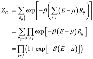 (9)
(9)
We can evaluate then the average number of links
 (10)
(10)
where P0 is the probability of occupation of a single link
 (11)
(11)
Notice the similarity of our “free” model to the Fermi-Dirac gas model. As 
 , all links are
equally occupied with probability . As
. As 
 , if
, if  all links are unoccupied, while for
 all links are occupied with unit probability. The average number of occupied links as a function of the temperature is shown in Figure 1, to be compared later with the corresponding quality of the complete model.
2.2.2. 
The full Hamiltonian is not amenable to exact analytic results, the main problem being the appearance of quadratic terms. To circumvent this problem we resort to a gaussian integration. Let us concentrate on the individual
term . By defining the column vector

Figure 1. Mean number of links  vs. b for l = 0 and for values of the energy E below and above the chemical potential μ. The points are Monte Carlo simulation results for systems of N = 50 nodes, the solid line represents the analytic results and the error bars represent the standard deviation of L.
 (12)
(12)
we obtain
 (13)
(13)
with A the 2 × 2 matrix
 (14)
(14)
Using well known Gaussian matrix integrals we may rewrite
 (15)
(15)
where now  appear as linear terms. Including all sites we obtain the full grand partition function ZG
 (16)
(16)
where the integration measure is
 (17)
(17)
Summing over all possible configurations amounts to include the possible values of Rij (1 and 0). We end up with
 (18)
(18)
2.3. Approximate Solutions
The expression above, Equation (18), allows to extract the behavior of ZG in limiting cases
1) When , or equivalently
 , the integration measure, Equation (17), forces all
  to remain close to zero. We obtain then
 (19)
(19)
where
 (20)
(20)
We conclude that at high temperature, since , the interaction is irrelevant and our interacting model is reproduced by the results offered by the free model (with l = 0).
2) In the case 
 and
and  the term
  dominates over unity and the integration for a single site is simplified to
 (21)
(21)
Including all sites we arrive at
 (22)
(22)
Thus at low temperatures the presence of the interaction amounts to a renormalization of the chemical potential
 (23)
(23)
The net result is that the interaction allows more links to be located under the Fermi energy with a high probability being occupied.
Mean-Field Approximation
For a network with a big number of links, we may resort to a mean field approximation, applicable to any temperature. The grand canonical partition function may be rewritten as
 (24)
(24)
For a large number of links we may approximate  and
and  by their mean values
 (25)
(25)
 (26)
(26)
where P is the occupation probability of a single link.
ZG becomes then
 (27)
(27)
The above expression is similar to the grand canonical partition function of the free model, with μ replaced by . We conclude that the occupation probability of a single link satisfies the equation
 (28)
(28)
We may attempt a numerical solution of the above equation. Let us define
 (29)
(29)
 (30)
(30)
The solution(s) of Equation (28), we call it P*, is found as the intersection of the two curves f1 and f2
 (31)
(31)
P ranges from 0 to 1, and while at P = 0 f2 lies below f1, at P = 1 f2 lies above f1. Thus f2 is forced to cross f1 at some point P*. For large values of b and l this crossing occurs more than once. Consider a Taylor expansion around the initial crossing point P*
 (32)
(32)
 (33)
(33)
When the slope of f2 is bigger than the slope of f1 at P*, then f2 rises above f1 for  and below f1 for
 . This implies that we will have two more crossing points (two more solutions), when the condition
 (34)
(34)
is satisfied. For a range of the parameters involved this crossing occurs more than once, giving rise to a bifurca-
tion [21] [22] . When , the initial P* is equal to
  and the bifurcation condition becomes
 (35)
(35)
2.4. Monte Carlo Algorithm
We performed Monte Carlo simulations of the above described system and compared them with our exact results. Monte Carlo simulations are usually performed for thermal systems using the canonical ensemble and the well known “Metropolis” algorithm. The grand canonical ensemble is much more difficult to simulate and not routinely used in the literature [23] . In the classic “Metropolis” method system configurations are generated from a previous state using a transition probability which depends on the energy difference between the initial and final states. The sequence of states produced follows a time ordered path, but the time in this case is “Monte Carlo time” and should not be confused with actual time. It is simply an effort to mimic a dynamic process that will lead the system to equilibrium so that statistical averages can be computed. Consider a discrete state-continuous time system. If  denotes the probability that a system is found at state n at time t and
  denotes the transition rate from state n to state m then the dynamics of the system are described by the following master equations (one for each of the discrete system states)
 (36)
(36)
In equilibrium . Thus, one obtains the “detailed balance” condition:
 (37)
(37)
For the canonical ensemble the probability to find the system at the n-th state is:
 (38)
(38)
From Equation (37) and Equation (38) one deduces that the ratio of the transition probabilities depends only on the energy difference between the states and not on the unknown Z function.
 (39)
(39)
The calculation of thermodynamical statistical averages would be trivial if we knew the partition function Z in Equation (38). Since this is, however, generally unknown in Monte Carlo simulations we start from a random system configuration and allow it to evolve with suitable chosen transition probabilities. Any choice of transition probabilities that satisfies Equation (38) is acceptable. The standard “Metropolis” algorithm consists in choosing
 (40)
(40)
The “Metropolis” algorithm briefly procceeds as follows:
1) Choose a random initial state m.
2) Choose a new state n from the “neighboring” states to state m.
3) Calculate the energy difference ΔE between the two states.
4) Draw a random number r uniformly distributed between 0 and 1.
5) Use Equation (39) to decide whether to accept the new state, i.e. accept if  or if
or if 
6) Return to Step 2.
The above equations are valid for systems with a fixed number of “particles” Np at constant temperature T.
An alternative way of studying physical systems is by using the grand canonical ensemble. In this case the number of “particles” of the system may vary i.e. the system can exchange particles with its environment. Thus, the independent variables are T and the chemical potential μ. For the grand-canonical ensemble the probability to find the system at the n-th state is:
 (41)
(41)
where ZG is the grand partition function, μ is the chemical potential and Np is the number of “particles” of the system.
One may think that simulating the grand canonical ensemble is a trivial extension of the above algorithm and that it suffices to use Equation (41) in the place of Equation (38), while calculating the acceptance probabilities. This is true in principle; however there are practical complications that should be considered. Consider for simplicity a spin system, i.e. a system where each particle can be found in one of two states (spin up or down) and that can exchange particles with its environment.
A rough sketch of the proper algorithmic process that should be used for a grand canonical simulation is as follows:
1) Choose at random a state i. This state has energy Ei and n particles.
2) Find all the “neighboring” states of i. This includes all the states accessible from i if we insert one particle, all states accessible from i if we remove one particle and all states resulting from a random spin flip (a rearrangement of the internal degrees of freedom). Select randomly one of these states.
3) Calculate the energy  and the number of particles
  of this trail state.
4) Calculate the acceptance ratio starting from Equation (41) instead of Equation (38). Accept or reject the trial state.
5) Continue until the system reaches a steady state.
In practice, Step 2 of finding the “neighboring” states can become rather complicated and “heuristic” tricks have to be implemented to simplify the process.
Our network system is a system with variable number of links L. We performed grand canonical Monte Carlo simulations of this system using the temperature T and chemical potential μ as control parameters using the following algorithm.
1) We start from a network of N nodes and we randomly insert L0 links out of the possible  with probability 1/2.
2) We calculate the energy of the system H and the number of links L.
3) We draw a random number x between 0 and 1. If  we try to transpose a link. If
  we try to remove a link. And if
  we try to insert a link in the system.
4) In case we decide to transpose a link then we generate a new trial configuration with just one link in a different “place”. We accept the new configuration with probability  where
where  and
and  the energy of the new configuration.
5) In the case of insertion we generate a new configuration with one additionally randomly placed link and accept the new configuration with probability  where
where ,
,
 the number of links of the new configuration and
  a correction term that accounts
for the difference in the number of available states when the number of links increases by one.
6) Links are removed with probability  where
where  and
and
 a correction term that accounts for the difference in the number of available states
when the number of links decreases by one.
7) We continue the simulation for a number of Monte Carlo steps which ensures that the system has reached equilibrium.
8) We repeat the calculations for several initial system realizations.
3. Results
In Figure 1 we plot the mean number of links  as a function of β for the case
 , after the system has reached the equilibrium state. The exact analytic results (solid lines) and the Monte Carlo simulations (points)
are in excellent agreement. We observe that for small β , the mean number of links tends to
 ,
,
while for large β there are two limits: for
 , the mean number of links tends to
  and for
  the mean number of links tends to zero. We notice here that the results are identical to the corresponding results from traditional statistical mechanics for systems of non-interacting fermions (Fermi-Dirac distribution).
In Figure 2 we present the results for the interacting case, with ,
,  , for different energies, as a function of β. Distinctive features emerge. First at high temperatures
  the occupation probability for a
link is always . This is in agreement with our findings in section 2.3, that at high temperatures the interaction
term is not important and the results are reproduced by the grand partition function of the free model. As β increases (temperature decreases) the results are sensitive upon the precise value of the energy. In Figure 2(a) the energy is smaller than the effective chemical potential. The probability starts to rise with increasing β (as expected) and at a critical β value the bifurcation takes place. The original solution becomes unstable and two new branch-solutions emerge. In Figure 2(b) on the other hand the energy is bigger than the effective chemical potential. As β increases, the probabiity decreases and again at a critical β value the bifurcation occurs. In Figure 2(c) the energy is equal to the effective chemical potential. The probability remains constant at the value
 and the bifurcation takes place at the predicted value
 . In Figure 3 we display characteristic pictures
of the network for both the free and the interacting case. We notice that in the free model there are very few connecting links. In the interaction model on the other hand, we obtain a very dense network.
What is really striking in our findings is the impressive agreement between the mean field approximation, Equation (28), and the Monte Carlo simulation we carried out (see all the figures). We attribute this agreement to the large number N of the sites involved. Our findings imply a sort of “equivalence” among all sites and therefore we do not expect the creation of hubs in the network.
4. Conclusions
We have studied a dynamical directional network model with a variable number of links. In most of similar studies

Figure 2. For l = 2 and μ = 2. The solid line represents mean-field approximation results and the points are Monte Carlo simulation results for systems of N = 50 nodes.

Figure 3. Characteristic pictures of the network for both the free (l = 0) and the interacting case (l = 0.49) for E = 1.4, μ = 1, b = 6 and N = 20 nodes.
the links are added or removed following a given prescription. In our model the number of links is affected by the presence of an interaction term in the Hamiltonian. The whole network pattern is sensitive upon the values of the strength of interaction l, the inverse temperature β and the chemical potential μ. Though the model is not simple, we manage to obtain a semi-analytic description. At high temperatures the dynamics of the network is described by the free model, while at low temperatures the determining parameter is the renormalized chemical potential . It is rather gratifying the nice agreement between the theoretical expectations and the Monte-Carlo simulation.
We consider our model as a prototype model, able to address different situations. Variation of the assumptions and the parameters involved may lead to distinct patterns. For example:
1) We assume the same energy for all links. We may examine the possibility that links connected to specific sites have a reduced energy. Then we anticipate the emergence of hubs. Such a structure may resemble the internet structure.
2) There is no geometry in the present model. We may envisage that the sites belong to a fixed geometry, for example a lattice. The interaction term in the Hamiltonian may stand for the propagation of a germ from a human organ to another, or the propagation of a fire in a forest.
3) We consider l as a constant. A space-dependent l (including negative values) will give rise to a cluster of multiple networks, or a “multiverse”.
Work along these lines is in progress.
References
- Peirce, C.S. (1870) Memoirs of the American Academy of Sciences, 9, 317-378. http://dx.doi.org/10.2307/25058006
- Peirce, C.S. (1880) American Journal of Mathematics, 3, 15-57. http://dx.doi.org/10.2307/2369442
- Nicolaidis, A. (2009) International Journal of Modern Physics A, 24, 1175-1183. http://dx.doi.org/10.1142/S0217751X09043079
- Misner, C.W., Kip, S. and Thorne, J.A. (1973) Gravitation. W. H. Freeman, San Francisco.
- Wheeler, J.A. (1980) Pregeometry: Motivations and Prospects. In: Marlow, A.R., Ed., Quantum Theory and Gravitation, Academic Press, New York, 1-11. http://dx.doi.org/10.1016/B978-0-12-473260-5.50005-X
- Penrose, R. (1971) Angular Momentum: An Approach to Combinatorial Space-Time. In: Bastin, T., Ed., Quantum Theory and Beyond, Cambridge University Press, Cambridge.
- Penrose, R. (1972) On the Nature of Quantum Geometry. In: Klauder, J., Ed., Magic Without Magic, Freeman, San Francisco, 333-354.
- Konopka, T., Markopoulou, F. and Smolin, L. Quantum Graphity [arXiv:hep-th/0611197].
- Konopka, T., Markopoulou, F. and Severini, S. (2008) Physical Review D, 77, Article ID: 104029. http://dx.doi.org/10.1103/PhysRevD.77.104029
- Ambjorn, J., Jurkiewicz, J. and Loll, R. (2004) Physical Review Letters, 93, Article ID: 131301. http://dx.doi.org/10.1103/PhysRevLett.93.131301
- Krioukov, D., Papadopoulos, F., Kitsak, M., Vahdat, A. and Boguna, M. (2010) Physical Review E, 82, Article ID: 036106. http://dx.doi.org/10.1103/PhysRevE.82.036106
- Strogatz, S.H. (2001) Nature, 410, 268-276. http://dx.doi.org/10.1038/35065725
- Albert, R. and Albert-László, B. (2002) Reviews of Modern Physics, 74, 47-97. http://dx.doi.org/10.1103/RevModPhys.74.47
- Dorogovtsev, S.N. and Mendes, J.F.F. (2002) Advances in Physics, 51, 1079-1187. http://dx.doi.org/10.1080/00018730110112519
- Newman, M.E.J. (2003) SIAM Review, 45, 167-256. http://dx.doi.org/10.1137/S003614450342480
- Barrat, A., Barthelemy, M. and Vespignani, A. (2008) Dynamical Processes on Complex Networks. Cambridge University Press, Cambridge. http://dx.doi.org/10.1017/CBO9780511791383
- Nicolaidis, A., Kosmidis, K. and Argyrakis, P. (2009) Journal of Statistical Mechanics: Theory and Experiment, 2009, Article ID: P12008. http://dx.doi.org/10.1088/1742-5468/2009/12/P12008
- Cohen, R. and Havlin, S. (2010) Complex Networks: Structure, Robustness and Function. Cambridge University Press, Cambridge. http://dx.doi.org/10.1017/CBO9780511780356
- Childs, A.M., Gosset, D. and Webb, Z. (2013) Science, 339, 791-794. http://dx.doi.org/10.1126/science.1229957
- Faccin, M., Johnson, T., Biamonte, J., Kais, S. and Migda, P. (2013) Physical Review X, 3, Article ID: 041007.
- Park, J. and Newman, M.E.J. (2004) Physical Review E, 70, Article ID: 066117. http://dx.doi.org/10.1103/PhysRevE.70.066117
- Park, J. and Newman, M.E.J. (2004) Physical Review E, 70, Article ID: 066146. http://dx.doi.org/10.1103/PhysRevE.70.066146
- Binder, K. and Heermann, D. (2010) Monte Carlo Simulation in Statistical Physics: An Introduction. Springer, Berlin.