Applied Mathematics
Vol.5 No.6(2014), Article ID:44596,8 pages DOI:10.4236/am.2014.56093
Influential Observations in Stochastic Model of Divisia Index Numbers with AR(1) Errors
Syed Muhammed Aqil Burney1, Arfa Maqsood2
1Department of AS&RM, College of Computer Science and Information Systems, Institute of Business Management Karachi, Pakistan
2Department of Statistics, University of Karachi, Karachi, Pakistan
Email: aqil.burney@iobm.edu.pk, amaqsood@uok.edu.pk
Copyright © 2014 by authors and Scientific Research Publishing Inc.
This work is licensed under the Creative Commons Attribution International License (CC BY).
http://creativecommons.org/licenses/by/4.0/


Received 31 December 2013; revised 31 January 2014; accepted 8 February 2014
ABSTRACT
We use the general form of hat matrix and DFBETA measures to detect the influential observations in order to estimate the Divisia price index number when the error structure is first order serial correlation. An example is presented with reference to price data of Pakistan. Hat values show the noteworthy findings that the corresponding weights of consumer items have large influence on the parameter estimates and are not affected by the parameter of autoregressive process AR(1). Whereas DFBETAs for Divisia index numbers depend on both the weights and autoregressive parameter.
Keywords:Hat Matrix, DFBETA, Divisia Index Number, Influential Observation, Autoregressive Process

1. Introduction
A number of studies are available on the detection of leverages and influential observations in a regression model when the errors are assumed to be serially correlated with AR(1) and AR(2) processes. For instance, initially, Prais and Winsten [1] , Kadiyala [2] , Girilches and Rao [3] , Maeshiro [4] , and Park and Mitchell [5] have observed the significant effect of the first observation on the parameter estimates of regression model. Influence diagnostics are developed and studied by many authors, including Belsley et al. [6] , Cook ([7] [8] ), Cook and Weisberg [9] , Draper and John [10] , and Draper and Smith [11] . They examined the effect of individual observation or a set of observations on the estimation of model parameters. The problem of influence diagnostic checking for the linear regression model with autocorrelated errors has, now, received much attention of the researchers and statisticians. Puterman [12] observed that the first transformed observation in linear regression model can have a large impact on the parameter estimates. Some authors agreed that the effect of not including the first observation is not always magnificent as suggested by Cochrane and Orcutt [13] . Stemann and Trenkler [14] extended the approach of Puterman [12] to the general linear model with the first order autoregressive errors and showed the effect of the presence of a constant term on a leverage point when the correlation of the error term was large in absolute value. Barry et al. [15] extended the study of influential observations to the regression model with AR(2) errors and developed the diagnostic techniques using a hat matrix.
Much literature is on hand on the influential observations diagnostic for the regression models with continuous type of regressors. There is a need to have some techniques for finding the influential observations when the dilemma of constructing the index number is concerned. The objective of this paper is to use the analytical tools of hat matrix and DFBETA measures to identify the influential observations in estimating the Divisia price index number.
The paper is organized as follows. Section 2 introduces the Divisia index number model and the role of the initial observation in estimation of model is discussed. The relevant concepts on influence diagnostics for the underlying model are presented in Section 3. An application with reference to Pakistan price data is illustrated in Section 4 and lastly, Section 5 recapitulates the results.
2. Regression Model
The well-known Divisia index number is formulated by the following model
 (1)
(1)
where , log price-change in period t for ith commodity,
  conman trend in the prices of all commodities at time t (the rate of inflation), and
  is the random component. The errors are assumed to be generated from the first order autoregressive scheme, that is
 , where
 , and
, and 
This yields the error structure of model (1) as
 and variance-covariance
  (2)
(2)
Defining more compactly in matrix notation as follows,

The inverse of variance-covariance matrix can easily be decomposed using cholesky decomposition and can be written as

where Q is a lower triangular matrix of order (nT × nT), defined as

The model (1) is written in matrix form
 (3)
(3)
It is well known that under the above assumption, the best linear unbiased estimator (BLUE) of  in model (1) could be obtained by the generalized least square (GLS) approach as given below

There are different approaches to estimate the parameter vector , in case of unknown autoregressive parameter
  (see Judge et al. [16] ). The value of
  is first estimated from the data using any of the number of suggested alternatives given in Gugarati [17] . The transformation of the vector
  and the design matrix
  to the new vector
  and matrix
  to obtain

where  are the vectors of one and zero respectively i.e.
  and
and . We can now apply the simple ordinary least square (OLS) estimator to the transformed data to obtain estimated generalized least square (EGLS) and we have
 (4)
(4)
Substituting the results in Equation (4) provides the estimator of , the familiar Divisia index numbers, written as
 (5)
(5)
3. Influence and Hat Matrix
Several measures and plots have been developed to detect the influential observations in linear regression. Hat matrix is one of the common quantity that is used in detecting the influential points when the OLS procedure for estimation of regression parameter is used. The quantity is

The hat matrix for the transformed data  is written as

The diagonal elements of the hat matrix, denoted by  or
or , are used as diagnostic technique for measuring the influence of a specific observation i on regression parameter estimates. The entries of matrix depend only on the values of design matrix X, and thus they serve as a measure of the distance of an observation from the centre of data. The large diagonal values indicate potentially large impact of the corresponding observation on regression estimates and thus considered an influential point if it satisfies the criteria that have the cut off points i.e.
 . We obtain the hat matrix for model (1) using the transformed matrix
  described in Section 2 as follows:
 (6)
(6)
The elements of matrix clearly show that the weights of commodities determine how much the important of particular commodity is in order to find the Divisia index number, and remain same for each time period t. They are not affected by the parameter of autoregressive process. The greater the value of weight, the more influential the commodity is, irrespective of the time period, because we are assuming the same weights over the underlying time period.
Another chief role of hat matrix in finding the significant expression to assess the effect of deleting an observation on parameter estimates and predicted values. The vector DFBETA, given by Belsley et al. [6] , which denotes the difference between the estimates of the vector  with and without the ith observation i.e.;
 (7)
(7)
where  is the estimate of
  with the ith observation excluded.
Puterman [12] studied the impact of the first observation in the constant mean model and regression through the origin model with AR(1) errors. One should see the work of Stemann and Trenkler [14] on the influence technique when considering the regression model with more than one regressors in the presence and absence of constant term. On the other hand, Barry et al. [15] extended the approach of Puterman to the influence of initial observations and subset of observations in linear regression model with AR(2) errors. Our main aim is, therefore, to obtain the influential points when we are dealing with index number model. For this purpose, we use equation (7) to find the results of DFBETA measures as follows;
 (8)
(8)
where p denotes the number of parameters in vector . It is clearly seen that the DFBETA values are affected by the autoregressive coefficient of AR(1) process. For t = 1, when
  increases to 1 in both positive and negative direction, deleting the ith observation has a great impact on the parameter estimates. When
 , all the entries of DFBETA matrix become zero that might reveal having the data with no influential point. Beside this all values depend on the constant factor of ith weight embodied by the first part of expression (8).
4. An Application
In this section, we present an application to price data for Pakistan. The data consists of 374 consumer items classified in ten groups for the period from July 2002 to June 2011. The groups are food and beverages, apparel textile and footwear, house rent, fuel and lighting, household furniture and equipment, transportation and communication, recreation and entertainment, education, cleaning laundry and per. appea, and medicare. In the first phase, we compute the parameter vector  using formula (5) which demonstrates the Divisia index number when the same weights are used through the entire period. To estimate the value of
 , the residuals versus observation numbers are plotted in Figure 1. The plot simply verifies the stationary scenario of time series with constant mean and constant variance.
The Durbin-Watson statistic is 1.4002, indicating the presence of autocorrelation in the residual series. The estimate of  using Yule-Walker procedure is obtained as 0.299. For each time period the hat values are estimated by the weights of commodities and large quantities are shown in Table 1. The highest hat entry is parallel to house rent index, implying its importance in estimating the index numbers. Others leading items include wheat flour bag, milk fresh, and electric charges for the consumption of more than 1000 units. To investigate the effect of presence of items with large hat values, we plot the estimated Divisia index numbers based on all items and without the items house rent and wheat flour bag in Figure 2. The index number estimates excluding house rent are much different from the estimates based on all items, whereas the estimates without wheat flour bag is relatively close to the index numbers with all observations.
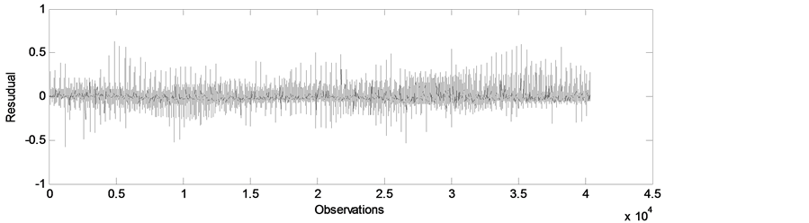
Figure 1. Plot of residual series.

Table 1. Significant hat values for the items exceeding cut-off value 0.005348.
Table 2 presents list of items with the significant DFBETAs exceeding the cutoff value 0.00995. The large values of  are represented by the values with superscript *. Out of these 37 influential items, 32 are from the first commodity group food and beverages that include wheat flour, vegetable ghee, sugar, beef with bones, and mutton with the corresponding higher diagonal values of hat matrix. Sugar refined with
  has an impact on estimation index number relating to 41 months or in other words, it affects the values of 41 alphas in parameter vector
 . Other influential commodity groups include house rent with the highest
 , fuel and lighting, and transportation and communication.
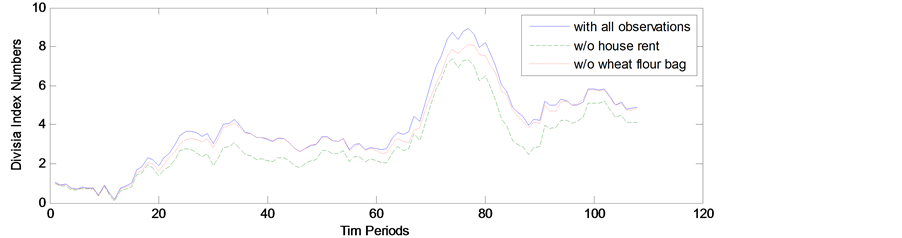
Figure 2. Divisia index numbers including all items, excluding house rent and wheat flour.
Table 2. Significant DFBETAs corresponding to items and their hat values.
Continued
5. Conclusion
In this paper, we use the general expression of hat matrix and DFBETA measure to detect the influential observations in order to estimate the Divisia price index number when the error is generated from AR(1) process. The hat values only depend on the weights of commodities, showing that the corresponding weights of consumer items have large influence on the parameter estimates and are not affected by the parameter of autoregressive process AR(1). An example is presented with reference to price data of Pakistan. From the findings of both hat matrix and DFBETAs, food and beverages are the leading commodity group as the maximum number of items in which group has large hat values and DFBETAs measures.
Acknowledgements
The authors are thankful to Dept. of Computer Science and Dept. of Statistics University of Karachi for providing computing and research facilities and Dr Ejaz Ahmed, Dean CCSIS ,Institute of Business Management Karachi for technical discussion and support.
References
- Prais, G.J. and Winsten, C.B. (1954) Trend Estimates and Serial Correlation. Cowles Commission Discussion Paper, Stat. No. 383, University of Chicago.
- Kadiyala, K.R. (1968) A Transformation Used to Circumvent the Problem of Autocorrelation. Econometrica, 36, 93-96. http://dx.doi.org/10.2307/1909605
- Griliches, Z. and Rao, P. (1969) Small-Sample Properties of Several Two-Stage Regression Methods in the Context of Autocorrelated Disturbances. Journal of American Statistical Association, 64, 253-272. http://dx.doi.org/10.1080/01621459.1969.10500968
- Maeshiro, A. (1979) On the Retention of the First Observation in Serial Correlation Adjustment of Regression Models. International Economic Review, 20, 259-265. http://dx.doi.org/10.2307/2526430
- Park, R.E. and Mitchell, B.M. (1980) Estimating the Autocorrelated Error Model with Trended Data. Journal of Econometrics, 13, 185-201. http://dx.doi.org/10.1016/0304-4076(80)90014-7
- Belsley, P.A., Kuh, E. and Welsch, R.E. (1980) Regression Diagnostics. John Wiley, New York. http://dx.doi.org/10.1002/0471725153
- Cook, R.D. (1977) Detection of Influential Observations in Linear Regression. Technometrics, 19, 15-18. http://dx.doi.org/10.2307/1268249
- Cook, R.D. (1979) Influential Observations in Linear Regression. Journal of American Statistical Association, 74, 169- 174. http://dx.doi.org/10.1080/01621459.1979.10481634
- Cook, R.D. and Weisberg, S. (1982) Residuals and Influence in Regression. Chapman and Hall, New York.
- Draper, N.R. and John, J.A. (1981) Influential Observations and Outliers in Regression. Technometrics, 23, 21-26. http://dx.doi.org/10.1080/00401706.1981.10486232
- Draper, N.R. and Smith, H. (1998) Applied Regression Analysis. 3rd Edition, John Wiley, New York.
- Puterman, M.L. (1988) Leverage and Influence in Autocorrelated Regression Model. Journal of the Royal Statistical Society, 37, 76-86.
- Cochrane, D. and Orcutt, G.H. (1949) Application of Least Squares Regression to Relationships Containing Autocorrelated Error Terms. Journal of American Statistical Association, 44, 32-61.
- Stemann, D. and Trenkler, G. (1993) Leverages and Cochrane-Orcutt Estimation in Linear Regression. Communication in Statistics-Theory and Methods, 22, 1315-1333. http://dx.doi.org/10.1080/03610929308831088
- Barry, A.M., Burney, S.M.A. and Bhatti, M.I. (1997) Optimum Influence of Initial Observatins in regression Models with AR (2) Errors. Applied Mathematics and Computations, 82, 57-65. http://dx.doi.org/10.1016/S0096-3003(96)00024-0
- Judge, G.G., Griffiths, W.E., Hill, R.C., Lutkepohl, H. and Lee, T.C. (1985) The Theory and Practice of Econometrics. 2nd Edition, John Wiley, New York.
- Gujarati, D.N. (2003) Basic Econometrics. 4th Edition, McGraw-Hill, New York.